In this post
- ADCP Technology: Why Acoustic Doppler Current Profilers Matter for Water Measurement
- What Is an ADCP? Full Form, Meaning, and How It Differs from a Point Current Meter
- ADCP Doppler Effect: How Sound Waves Measure Water Velocity?
- ADCP Flow Measurement: Beam Geometry, Janus Configuration, and Velocity Calculation
- ADCP Frequency Guide: 300 kHz vs 600 kHz — Range, Resolution, and Depth Trade-offs
- ADCP Components Explained: Transducers, Sensors, Signal Processor, and Housing
- ADCP Accuracy and Data Quality: Common Errors, Noise Sources, and How to Fix Them
- ADCP vs. Mechanical Current Meters, Single-Point Meters, and Electromagnetic Sensors
- ADCP Applications: River Discharge Measurement, Ocean Current Surveys, and Offshore Engineering
- Choosing the Right ADCP — The Oceantek Product Family
- Frequently Asked Questions (FAQ)
1. ADCP Technology: Why Acoustic Doppler Current Profilers Matter for Water Measurement
Imagine standing on a bridge over a river. You can see the water’s surface moving, but you have no way of knowing how fast the water is flowing three meters down — let alone at the very bottom. In the ocean, the challenge multiplies: currents shift direction layer by layer, driven by tides, density gradients, and wind. Understanding this three-dimensional flow field is not academic — it underpins flood forecasting, safe navigation, offshore construction, and climate research.
An Acoustic Doppler Current Profiler (ADCP) solves this problem in a single instrument package. It sends pulses of sound into the water column and listens to the echoes returning from particles and plankton drifting with the flow. By measuring the Doppler frequency shift at each time slice — corresponding to each depth layer — it reconstructs a complete current velocity profile from near-surface to near-bed, all without any moving parts in the water.
This article is written for hydrologists, oceanographers, engineers, and students who want more than a surface-level explanation. We will cover the precise physics of Doppler current measurement, the engineering behind Janus beam geometry, signal processing strategies, frequency selection trade-offs, common sources of measurement error, and how to connect these technical details to real decisions — like whether a direct-reading ADCP for a moving-boat survey or a self-contained ADCP for a year-long mooring is the right tool. As a manufacturer that designs and builds ADCPs in-house, Oceantek provides this deep-dive so you can choose and operate your instrument with confidence.
2. What Is an ADCP? Full Form, Meaning, and How It Differs from a Point Current Meter
1.1 A Short History of Acoustic Current Measurement
The conceptual roots of ADCP technology trace back to the 1960s, when oceanographers began experimenting with acoustic backscatter to remotely sense water motion. The first practical vessel-mounted ADCP was developed in the late 1970s by Fran Rowe and Kent Deines at RD Instruments (RDI) in San Diego. Their breakthrough was the realization that by using multiple acoustic beams in a symmetrical Janus configuration, the three-dimensional velocity vector could be reconstructed without needing to know the exact speed of sound at every depth — the symmetry cancels first-order errors.
Since then, ADCPs have evolved from specialized research tools weighing over 100 kg into compact, commercially available instruments. Modern solid-state electronics, broadband coding, and phased-array transducer technology — all of which Oceantek incorporates into its product line — have reduced power consumption, improved velocity precision, and expanded profiling range to over 1,000 meters.
2.2 What Makes an ADCP Different from a Point Current Meter?
A single-point current meter — whether mechanical (rotor), electromagnetic, or acoustic — measures velocity at one location. To obtain a profile across the water column, you would need to deploy multiple instruments at different depths simultaneously, which is expensive, logistically complex, and introduces inter-instrument calibration issues.
An ADCP, by contrast, measures the entire velocity profile in one deployment. This is what the term “profiler” refers to: the instrument divides the water column into discrete depth bins (cells) and reports a velocity vector for each one, from a blanking distance just in front of the transducer face out to the maximum profiling range. For hydrologists, this means a single moving-boat ADCP transect can compute total river discharge in minutes — a task that once took hours with mechanical current meters lowered from a cableway.
| Feature | Single-Point Current Meter | ADCP |
|---|---|---|
| Measurement volume | One location | Entire water column (up to 255 depth cells) |
| Velocity components | 2D or 3D at a single point | 3D velocity profile (East, North, Up) |
| Discharge measurement | Requires multiple instruments or vertical traversing | Moving-boat method; discharge computed in real time |
| Moving parts | Rotors (mechanical type) | None — all solid-state acoustic |
| Deployment duration | Days to weeks (battery-limited) | Up to 12+ months (self-contained models) |
2.3 The Four Core ADCP Configurations
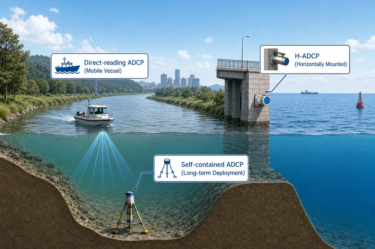
All ADCPs share the same underlying measurement principle, but they are packaged differently for different operational needs:
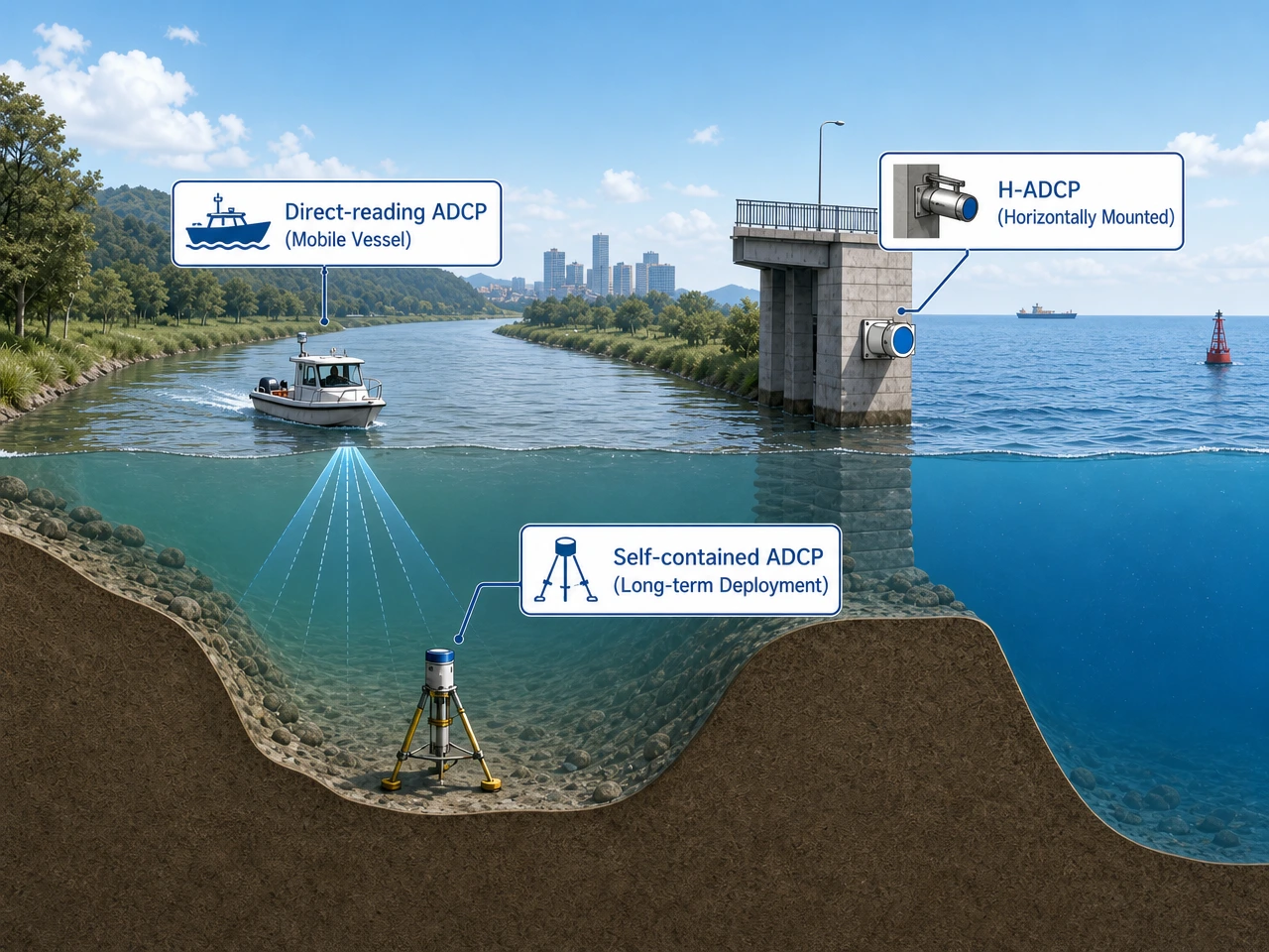
- Direct-reading (Real-time) ADCPs: Connected via cable to a surface computer or data logger. Ideal for moving-boat discharge surveys, vessel-mounted oceanographic profiling, and any application where you need immediate data feedback. Oceantek’s direct-reading models stream ensemble-averaged velocity profiles to your laptop in real time.
- Self-contained (Autonomous) ADCPs: Battery-powered with internal solid-state memory. Deployed on seabed frames or moorings for weeks to months, recording data internally for retrieval. These are the workhorses of long-term oceanographic monitoring.
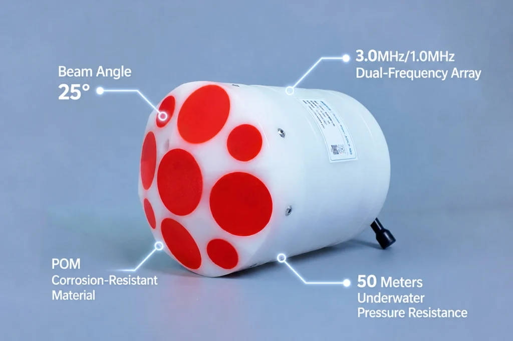
- River-type ADCPs: Optimized for shallow-water hydrology with higher frequencies (600 kHz to 3,000 kHz) for finer depth resolution. They often include specialized discharge-measurement software and GPS integration for moving-boat surveys.
- Horizontal ADCPs (H-ADCP): Permanently installed on a riverbank, bridge pier, or channel wall, beaming horizontally across the flow. They provide continuous, real-time index-velocity data for flood warning, irrigation management, and dam operations — 24/7, 365 days a year.
3. ADCP Doppler Effect: How Sound Waves Measure Water Velocity?
3.1 The Classical Doppler Principle
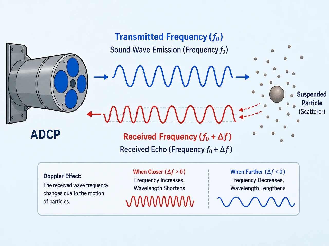
The Doppler effect — named after Austrian physicist Christian Doppler, who described it in 1842 — is the change in observed frequency when a wave source and a reflector move relative to each other. It is the same physics that makes an ambulance siren sound higher-pitched as it approaches you and lower-pitched as it drives away.
In the ADCP context, the “source” is the instrument’s transducer, which emits an acoustic pulse at a known transmit frequency ft. The “reflector” is a collection of suspended particles — sediment, plankton, bubbles — drifting passively with the water. When the sound wave strikes these particles, a portion of the acoustic energy scatters back toward the transducer. If the water (and therefore the scatterers) is moving toward or away from the instrument, the frequency of the returned echo fr will be shifted relative to ft.
3.2 The ADCP Doppler Equation
The fundamental relationship is given by:
fd = fr − ft = −2 · ft · (vr / c)Where:
- fd = Doppler frequency shift (Hz)
- ft = Transmitted acoustic frequency (Hz)
- fr = Received acoustic frequency (Hz)
- vr = Radial velocity of scatterers along the beam axis (m/s). Positive when moving toward the transducer.
- c = Speed of sound in water (typically ~1,500 m/s in seawater at 20°C, salinity 35 psu)
The factor of 2 accounts for the round-trip Doppler shift: the transmitted pulse undergoes one shift when it strikes the moving scatterer (scatterer as moving observer), and a second shift when the scattered energy is re-radiated (scatterer as moving source). Both shifts are in the same direction, doubling the effect.
3.3 Worked Numerical Example
To make this concrete: a 600 kHz ADCP measuring a water velocity of 1.0 m/s along the beam axis would produce a Doppler shift of:
fd = −2 × 600,000 Hz × (1.0 m/s ÷ 1,500 m/s)
fd = −2 × 600,000 × 0.000667
fd = −800 Hz
The ADCP’s signal processor must detect this 800 Hz shift on top of a 600,000 Hz carrier — a precision of about 1.3 parts per thousand. This is well within the capability of modern digital signal processing, which can resolve frequency shifts of a few Hz using autocorrelation techniques.
3.4 Three Critical Assumptions and Their Real-World Validity
The Doppler current measurement method rests on three assumptions. No natural environment satisfies them perfectly, but decades of field validation show the measurement remains robust:
- Passive drift: Scatterers move at the same velocity as the surrounding water. Limitation: Large particles or organisms may have their own swimming or settling velocity. In practice, the vast majority of naturally occurring scatterers — fine sediment, phytoplankton, microscopic zooplankton — are small enough that their Stokes settling velocity is negligible (< 1 mm/s).
- Homogeneous flow across the beam footprint: The velocity is uniform across the horizontal extent of each beam at a given depth. Limitation: In highly turbulent or sheared flows, the four beams may sample slightly different water masses. The Janus configuration and ensemble averaging (Section 3) mitigate this.
- Stable speed of sound: The speed of sound c does not vary significantly over the profiling range. Limitation: Sound speed depends on temperature, salinity, and pressure. ADCPs compensate by measuring temperature at the transducer and, in some models, computing a sound speed profile from auxiliary CTD data.
4. ADCP Flow Measurement: Beam Geometry, Janus Configuration, and Velocity Calculation
4.1 Beam Geometry and the Janus Configuration
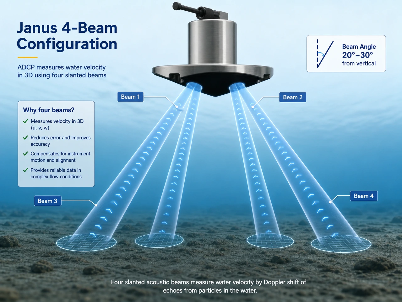
A single acoustic beam can only measure the velocity component along its own axis — the radial velocity. To reconstruct the full three-dimensional current vector (East, North, Up), an ADCP needs at least three beams pointing in different, non-coplanar directions. Most ADCPs, including every Oceantek model, use four beams in what is known as the Janus configuration.
In a Janus array, four beams are arranged in two orthogonal coplanar pairs, each beam tilted at a fixed angle (typically 20° or 30°) from the vertical axis. Looking down from above, the beams form an “X” pattern. This geometry confers two powerful advantages:
- Error cancellation: If the instrument tilts or pitches — as happens on a moving boat — the errors in the along-beam velocity measurements are equal and opposite in the paired beams. When the beam velocities are combined to compute Earth-coordinate currents, the tilt-induced errors largely cancel. This is why a vessel-mounted ADCP can produce high-quality velocity profiles even in moderate sea states.
- Redundancy: Four beams provide one more radial velocity measurement than the minimum of three needed for a 3D solution. This redundancy — known as error velocity — serves as a real-time quality indicator. If the error velocity is large, it signals that the assumption of homogeneous flow is breaking down, alerting the operator to potential data quality issues.
4.2 Range Gating — How an ADCP “Sees” at Different Depths
The ADCP does not measure all depths simultaneously. It transmits a short acoustic pulse — typically lasting a few hundred microseconds — and then switches to receive mode, listening to the returning echo over time. Because sound travels at a known speed through water, the arrival time of each segment of the echo corresponds to a specific distance from the transducer:
Range = (c × Time) / 2(Again, the division by 2 accounts for the round trip — sound travels to the scatterer and back.)
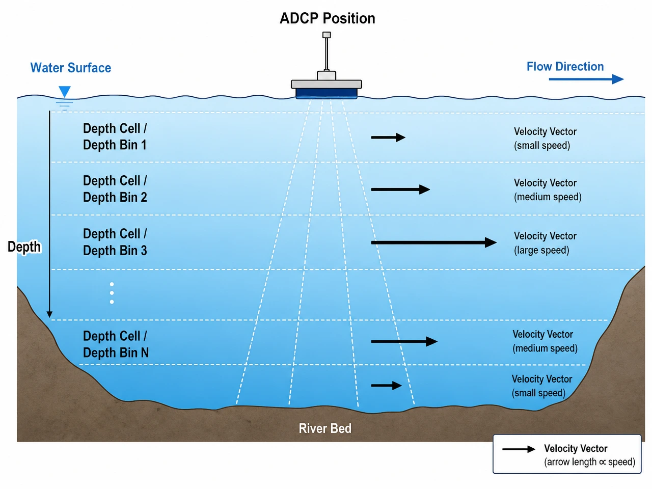
The receiving electronics divide the continuous echo into a series of consecutive time windows, or range gates. The Doppler shift is computed independently for each gate, yielding a velocity measurement at each corresponding depth. The resulting data product is a series of depth bins (also called depth cells), each with its own East, North, and Up velocity component.
The operator can configure:
- Depth cell size: Typically 0.1 m to 8 m, depending on the application. Smaller cells give finer vertical resolution but reduce the maximum profiling range (because each cell contains less scattered energy).
- Number of depth cells: Up to 255, defining the total profiling range = blanking distance + (cell size × number of cells).
- Blanking distance: A short zone immediately in front of the transducer face where measurements are not made. This allows the transducer to finish ringing after the transmit pulse and avoids near-field effects.
4.3 Coordinate Transformation — From Beam to Earth Coordinates
The raw output from an ADCP is four radial (along-beam) velocities — one from each transducer. Converting these to real-world current measurements involves a sequence of coordinate transformations:
- Beam → Instrument coordinates: Using the known beam geometry (the Janus angle, typically 20° or 30°), the four radial velocities are combined through a transformation matrix to yield three orthogonal velocity components in the instrument’s own frame of reference — plus the error velocity (the redundant fourth measurement).
- Instrument → Earth coordinates: The instrument-frame velocities are rotated into geographic coordinates (East, North, Up) using real-time data from the internal tilt sensor (pitch and roll) and fluxgate compass (heading). This step corrects for any tilt or rotation of the instrument housing.
- Vessel motion correction (bottom-tracking or GPS): For moving-boat surveys, the ADCP measures water velocity relative to the instrument. To obtain absolute water velocity, the instrument’s own motion over the ground must be subtracted. This is done using either:
- Bottom-tracking: A separate, longer acoustic pulse that reflects off the riverbed or seabed. By measuring the Doppler shift of the bottom echo, the ADCP can determine its own speed over ground independently. This works in water depths up to the bottom-tracking range limit.
- Differential GPS: Required when the water depth exceeds the bottom-tracking range (e.g., deep ocean profiling). GPS antennas at known offsets from the ADCP provide vessel course-over-ground and speed-over-ground.
- Ensemble averaging: A single acoustic ping produces an inherently noisy velocity estimate because of the random distribution of scatterers in the water. To achieve usable accuracy, many pings — typically tens to hundreds — are transmitted in rapid succession, and the results are averaged into an ensemble lasting from about 0.5 seconds (for highly dynamic flows) to 10 minutes (for deep, slowly varying ocean currents). The standard deviation of the ensemble-averaged velocity decreases as 1/√N, where N is the number of pings — averaging 100 pings reduces random noise by a factor of 10 compared to a single ping.
4.4 Signal Processing — Narrowband vs. Broadband ADCP
An important distinction that directly affects measurement precision is the type of acoustic coding used:
| Parameter | Narrowband ADCP | Broadband ADCP |
|---|---|---|
| Transmit pulse | Single-frequency tone burst | Phase-encoded pseudorandom sequence |
| Velocity precision (single ping) | ~10–30 cm/s | ~1–5 cm/s |
| How it works | Measures mean frequency shift of the returned tone | Autocorrelation of the phase-coded return; measures phase change between successive coded pulses |
| Max profiling range | Longer (more energy per pulse) | Shorter for the same frequency (lower peak power) |
| Best for | Deep ocean profiling where range matters more than precision | High-resolution river discharge, turbulence studies, coastal surveys |
| Oceantek implementation | Available in 75 kHz deep-water models | Standard in 300 kHz, 600 kHz, and river-type ADCPs |
Broadband signal processing — which Oceantek uses across most of its product line — achieves a dramatic reduction in measurement noise by transmitting a coded pulse and computing the autocorrelation of the returned signal. For the same averaging interval, a broadband ADCP can achieve velocity standard deviations 5–10 times lower than a narrowband system, or equivalently, the same precision in 1/25th to 1/100th of the time. This is why modern river-discharge ADCPs can produce accurate results from a single boat transect.
5. ADCP Frequency Guide: 300 kHz vs 600 kHz — Range, Resolution, and Depth Trade-offs
One of the most common questions from first-time ADCP users is: “Which frequency should I choose?” The answer involves a fundamental trade-off between profiling range and spatial resolution, governed by the physics of acoustic attenuation in water.
5.1 The Acoustic Attenuation Trade-off
Sound attenuates (loses energy) as it travels through water due to absorption and spreading. Higher frequencies attenuate more rapidly than lower frequencies. The absorption coefficient α scales approximately with the square of frequency — so doubling the frequency roughly quadruples the absorption loss.
However, higher frequencies also provide better spatial resolution: the acoustic wavelength λ = c / f determines the minimum resolvable velocity cell size, and shorter wavelengths produce stronger scattering from smaller particles, improving the signal-to-noise ratio at short range.
5.2 Oceantek ADCP Frequency Selection Guide
| Frequency | Typical Max Profiling Range | Typical Depth Cell Size | Best Applications | Oceantek Models |
|---|---|---|---|---|
| 75 kHz | 550–650 m | 4–32 m | Deep-ocean current profiling, open-ocean moorings, basin-scale circulation studies | Direct-reading & Self-contained 75 kHz |
| 300 kHz | 120–160 m | 1–8 m | Coastal oceanography, continental shelf surveys, offshore wind farm site assessment, medium-depth moorings | Direct-reading & Self-contained 300 kHz |
| 600 kHz | 55–70 m | 0.5–4 m | River discharge measurement, estuary surveys, harbor and coastal engineering, H-ADCP fixed installations | HADCP-600, Direct-reading 600 kHz |
| 3,000 kHz | 0.06–40 m | 0.02–4 m | Very shallow streams, small channels, near-boundary layer measurements | River-ADCP-M9 (multi-frequency) |
Practical rule of thumb: The maximum profiling range in meters is approximately 1/10th to 1/5th of the frequency in kHz for typical environmental conditions. A 600 kHz ADCP profiles to ~50–75 m; a 300 kHz ADCP to ~150–250 m. Lower scatterer concentrations (very clear water) will reduce these ranges; higher concentrations (turbid rivers) may extend them slightly.
5.3 The Multi-Frequency Advantage
The Oceantek River-ADCP-M9 takes a different approach: it integrates three frequency arrays — 3,000 kHz (4 beams), 1,000 kHz (4 beams), and 500 kHz (1 vertical beam) — into a single instrument. The onboard processor automatically selects the optimal frequency based on real-time depth and scattering conditions. In shallow, narrow streams, it uses the higher frequencies for fine resolution; as the boat moves into deeper water, it switches to lower frequencies for longer range. The single 500 kHz vertical beam provides an independent depth measurement and surface tracking.
6. ADCP Components Explained: Transducers, Sensors, Signal Processor, and Housing
An ADCP is a tightly integrated system of acoustic, electronic, and mechanical subsystems. Understanding each component helps with installation planning, troubleshooting, and recognizing what differentiates one instrument from another.
6.1 Piezoelectric Transducers
The transducer is the “voice” and “ears” of the ADCP. It is made from piezoelectric ceramic (typically lead zirconate titanate, PZT), a material that physically deforms when an electric voltage is applied — and conversely, generates a voltage when deformed by incoming sound pressure. Each beam of the Janus array has its own dedicated transducer element. The ceramic geometry — diameter, thickness, and shape — is precision-engineered to the operating frequency and beam pattern: a larger-diameter element produces a narrower beam, which improves spatial resolution at range but increases the transducer head size. Oceantek transducers are computer-modeled and tank-tested to optimize the beam pattern for each frequency.
6.2 Electronic Signal Processor and Transceiver
The electronic subsystem performs several critical functions:
- Transmit waveform generation: Synthesizes the coded transmit pulse — whether a simple tone burst (narrowband) or a phase-encoded pseudorandom sequence (broadband).
- Receiver and analog-to-digital conversion: Amplifies the weak returned echo (typically nanovolts to microvolts at the transducer terminals), filters out-of-band noise, and digitizes the signal at high sample rates.
- Digital signal processing (DSP): The core computation — autocorrelation, spectral analysis, or pulse-pair processing to extract the Doppler frequency shift from the noisy received signal. Modern DSP chips perform this computation in real time for all depth cells across all four beams.
- Data formatting and output: Assembles processed velocity data into ensembles, appends time stamps and sensor data, and streams the output via serial, Ethernet, or internal storage.
6.3 Auxiliary Sensors
An ADCP is more than just an acoustic instrument — the following sensors are essential for converting raw beam velocities into accurate, georeferenced current data:
| Sensor | What It Measures | Why It Matters | Typical Accuracy (Oceantek) |
|---|---|---|---|
| Pressure sensor | Hydrostatic pressure → instrument depth | Essential for knowing which depth bin corresponds to which absolute depth; also records tidal elevation changes during long deployments | ±0.1% of full scale |
| Temperature thermistor | Water temperature at transducer face | Temperature is the dominant control on sound speed (1°C ≈ 4 m/s change in c). Accurate temperature compensation is essential for range-gating calculations. | ±0.1°C |
| Tilt sensor (accelerometer) | Pitch and roll angles | Required for the beam-to-Earth coordinate transformation. Without tilt correction, a 5° tilt in a 1 m/s current causes ~8.7 cm/s velocity error. | ±0.5° (static) |
| Fluxgate compass | Magnetic heading | Orients the instrument-frame velocity components to geographic North. Must be calibrated for the local magnetic environment (especially important near steel structures). | ±2° (after calibration) |
6.4 Housing and Mechanical Design
The pressure housing protects the electronics and transducers from the marine environment. Oceantek housings are machined from hard-anodized aluminum alloy (for depths to 1,500 m) or titanium alloy (for depths to 6,000 m). The housing design must balance conflicting requirements: sufficient wall thickness for pressure resistance, good thermal conductivity to dissipate heat from the electronics, and corrosion resistance for long-term seawater exposure. All Oceantek housings incorporate sacrificial zinc anodes for cathodic protection during extended deployments.
7. ADCP Accuracy and Data Quality: Common Errors, Noise Sources, and How to Fix Them
No measurement is perfect, and ADCP data carries several known error sources. A good operator recognizes these and either corrects for them or knows when data should be flagged as suspect. Below are the main error categories and practical mitigation strategies.
7.1 Random Noise and Ensemble Averaging
As discussed in Section 3.4, single-ping velocity estimates are noisy. The solution is ensemble averaging. For a broadband ADCP operating at 600 kHz, a 1-second ensemble of ~40 pings typically achieves a velocity standard deviation of ~1–3 cm/s. Increasing the ensemble interval to 60 seconds reduces this to a few mm/s — but at the cost of temporal resolution. The operator must choose the ensemble interval to match the time scales of interest.
7.2 Side-Lobe Interference
Acoustic beams are not perfectly collimated — they have side lobes (off-axis acoustic energy). In a Janus configuration, the main lobe of each beam points 20°–30° from vertical, but a small fraction of the acoustic energy is directed along other angles. When a side lobe intersects the water surface or the seabed, the strong reflection from these boundaries contaminates the velocity measurement in the depth cells near that boundary.
The practical impact: the deepest ~6–15% of the profile (depending on beam angle) is unreliable because of side-lobe interference with the bottom. An ADCP with a 20° Janus angle loses ~6% of range to this effect; a 30° ADCP loses ~15%. This is why the Janus angle itself represents a design trade-off: wider angles give better vertical velocity resolution but lose more near-boundary data.
7.3 Ambiguity Velocity
When the water velocity along a beam exceeds a certain threshold — the ambiguity velocity — the phase measurement “wraps around” and the ADCP reports a velocity in the opposite direction (aliasing). This is the acoustic equivalent of a car wheel appearing to spin backward in a video. The ambiguity velocity depends on the transmit frequency and the pulse coding scheme. For a typical broadband ADCP at 600 kHz, the ambiguity velocity is around ±5–10 m/s — well above most natural currents. However, in very fast tidal channels or near dam spillways, operators should check the instrument’s ambiguity limit.
7.4 Compass Errors and Magnetic Interference
The internal fluxgate compass measures the ambient magnetic field to determine heading. Near steel-hulled vessels, reinforced concrete structures, or subsea pipelines, the local magnetic field may be significantly distorted, introducing heading errors of 10° or more. A 10° heading error in a 1 m/s current translates to a cross-track velocity error of ~17 cm/s. For vessel-mounted surveys, using a GPS-based heading solution (dual-antenna GPS) bypasses this entirely. For moored deployments, compass calibration at the deployment site and careful site selection away from magnetic infrastructure are essential.
7.5 Sound Speed Errors
The range-gating calculation (depth = c × time / 2) depends on an accurate value for the speed of sound c. In seawater, c varies from about 1,450 m/s (cold, fresh) to 1,560 m/s (warm, saline). A 1% error in c produces a 1% error in the depth assigned to each velocity cell and a ~2% error in the velocity magnitude. Oceantek ADCPs measure temperature at the transducer and apply a standard sound-speed formula (e.g., Chen-Millero or Del Grosso). For the highest accuracy in stratified waters, a CTD profile can be uploaded to the ADCP to provide depth-dependent sound speed correction.
Quick Data Quality Checklist for Field Operators
- ✅ Check error velocity — consistently high values (> 0.1 m/s) indicate flow inhomogeneity or instrument issues.
- ✅ Check echo intensity (backscatter) profile — a smooth decay with range is normal; sudden drops suggest clear water or range limits.
- ✅ Check percent-good (the fraction of pings in an ensemble that passed quality thresholds) — values below 80% warrant investigation.
- ✅ Verify bottom-tracking lock (for moving-boat surveys) — loss of bottom track in the middle of a transect invalidates the discharge calculation.
- ✅ Monitor pitch/roll during the survey — sustained tilt > 5° degrades accuracy and may indicate mounting issues.
8. ADCP vs. Mechanical Current Meters, Single-Point Meters, and Electromagnetic Sensors
ADCPs are not the only way to measure water velocity. Choosing the right tool requires understanding how ADCPs compare with alternative technologies.
| Method | Principle | Profile or Point? | Key Advantage | Key Limitation | Typical Accuracy |
|---|---|---|---|---|---|
| ADCP | Acoustic Doppler (remote sensing) | Full profile | Complete water-column coverage from a single deployment; no moving parts | Side-lobe interference near boundaries; requires scatterers in water | ±0.5–1% of water velocity ± 2–5 mm/s |
| Mechanical current meter (rotor / propeller) | Rotation rate of a propeller or rotor in the flow | Point | Simple, well-established; low cost | Moving parts susceptible to fouling and wear; measures only at one depth; slow response to turbulence | ±1–2% of reading |
| Electromagnetic (EM) current meter | Faraday’s law — voltage induced by water moving through a magnetic field | Point | No moving parts; works in very turbid water; measures 2D velocity | Point measurement only; requires electrodes in contact with water; zero-drift over time | ±1–2 cm/s |
| Acoustic Doppler Velocimeter (ADV) | Acoustic Doppler (remote sensing) | Point (small sampling volume ~1 cm³) | Very high spatial and temporal resolution; ideal for turbulence measurements | Point measurement only; very short range (a few cm from probe); fragile in debris-laden water | ±0.5% of velocity ± 1 mm/s |
| HF Radar (CODAR / WERA) | Bragg scattering of HF radio waves off ocean wave crests | Surface only (~0.5 m depth) | Covers very large areas (tens of km); shore-based, no in-water hardware | Surface current only; spatial resolution is coarse (0.5–6 km); requires calibration | ±5–10 cm/s |
| Drifters / Floats | Lagrangian — track the trajectory of a drifting object | Single depth (or profiler for Argo floats) | Direct measurement of water parcel trajectories; long-range coverage | Sparse spatial/temporal sampling; drifts with the flow (not fixed-location); expensive per data point | Varies with positioning method |
Bottom line: ADCPs occupy a unique niche — they are the only practical method for obtaining fixed-location, time-series velocity profiles across the full water column without requiring multiple instruments. For most hydrological and oceanographic monitoring applications, they are the instrument of choice.
9. ADCP Applications: River Discharge Measurement, Ocean Current Surveys, and Offshore Engineering
9.1 River Discharge Measurement (Moving-Boat Method)
The moving-boat ADCP method has become the global standard for river gauging, endorsed by the USGS, the ISO (ISO 748), and national hydrological agencies worldwide. The procedure is straightforward: the ADCP is mounted on a small boat (or a remotely operated tethered platform) and traversed from one bank to the other. During the transect, the ADCP profiles velocity from near-surface to near-bed while bottom-tracking provides the boat’s course and speed over ground. The discharge-computation software integrates velocity across the cross-section and along the transect path in real time, yielding total discharge (m³/s) before the boat reaches the far bank.
Compared to the traditional mechanical current-meter method — which required lowering a meter at 20–30 verticals across the river, measuring at multiple depths at each vertical, and taking hours to process data — the moving-boat ADCP completes a discharge measurement in 10–20 minutes with comparable or better accuracy.
9.2 Fixed Horizontal Monitoring (H-ADCP) for Flood Warning
In rivers that require continuous discharge monitoring — for flood early warning, reservoir operations, or inter-basin water transfers — a Horizontal ADCP (H-ADCP) is permanently mounted on a bank or pier, beaming horizontally across the channel at a fixed depth. It measures an index velocity — the along-beam velocity at that specific location and depth — which is empirically correlated to the cross-section mean velocity (usually through periodic moving-boat ADCP calibration surveys). Once the index-velocity relationship is established, the H-ADCP provides a continuous, real-time discharge record with updates every few minutes, feeding directly into SCADA or hydrological telemetry networks.
The Oceantek HADCP-600 is purpose-built for this application, with a rugged housing rated for permanent immersion, low power consumption (suitable for solar-powered installations), and communication protocols compatible with standard hydrological data loggers.
9.3 Coastal and Estuarine Oceanography
Bottom-mounted, upward-looking ADCPs deployed on the seabed for weeks to months capture the full richness of coastal current dynamics — tidal ellipses, residual circulation, wind-driven upwelling events, and density-driven estuarine exchange flows. Because the ADCP records the entire vertical profile, researchers can separate barotropic (depth-uniform) and baroclinic (depth-varying) components of the flow, which is essential for understanding estuarine salt-wedge dynamics and sediment trapping.
9.4 Offshore Engineering and Renewable Energy
Before installing an offshore wind turbine, subsea pipeline, or tidal energy converter, engineers need to characterize the local current regime. ADCPs deployed on seabed frames provide multi-month current data used to compute extreme-value statistics (50-year return currents), fatigue-loading spectra, and operational weather windows. The three-dimensional nature of ADCP data is particularly valuable for tidal turbine siting, where small variations in flow direction and vertical shear across the rotor disk significantly affect power output predictions.
9.5 Ship-Mounted Ocean Current Surveys
Vessel-mounted ADCPs are standard equipment on oceanographic research vessels. They continuously profile currents beneath the ship while underway, building up transects of upper-ocean velocity across hundreds of kilometers. This capability is central to studies of western boundary currents (e.g., the Gulf Stream, Kuroshio), equatorial current systems, and Antarctic Circumpolar Current transport. With a 75 kHz ADCP, researchers can routinely profile to 700–1,000 m depth from a moving ship, providing a three-dimensional view of ocean circulation that would be impossible to obtain with any other single instrument.
10. Choosing the Right ADCP — The Oceantek Product Family
Selecting an ADCP comes down to answering three questions:
- What is the water depth at your site? This determines the frequency (Section 4) and whether you need bottom-tracking capability.
- Do you need real-time data or autonomous recording? This determines whether a direct-reading (cabled) or self-contained (battery + memory) model is appropriate.
- Is the deployment mobile or fixed? Vessel-mounted, shore-mounted, or moored — each has different mechanical and communication requirements.
Oceantek’s product line maps directly onto these use cases:
Direct-Reading ADCPs
For real-time surveys
- Cable-connected to surface computer
- Real-time velocity profiles and discharge
- Ideal for moving-boat gauging and vessel-mounted profiling
- Available in 300 kHz, 600 kHz
Self-Contained ADCPs
For long-term autonomous deployment
- Internal battery and solid-state memory
- Months to 1+ year unattended operation
- Ideal for seabed moorings and buoy deployments
- Available in 75 kHz, 300 kHz, 600 kHz
River & H-ADCP
For hydrology and fixed sites
- River-ADCP-M9: Multi-frequency (3,000/1,000/500 kHz)
- HADCP-600: Horizontal fixed-installation ADCP
- Optimized for shallow-water hydrology
For detailed specifications, velocity accuracy, profiling range limits, and physical dimensions across all models, visit the Oceantek Products Page. Our application engineers can help you select the optimal ADCP configuration for your specific field program — whether it’s a single moving-boat survey instrument or a fleet of long-term monitoring stations.
11. Frequently Asked Questions (FAQ)
ADCP stands for Acoustic Doppler Current Profiler. It is a hydroacoustic instrument that measures water current velocities across the entire water column using the Doppler effect — the shift in sound frequency when acoustic signals reflect off particles moving with the water.
An ADCP transmits short pulses of high-frequency sound from four (or more) angled beams arranged in a Janus configuration. Particles and plankton drifting in the water reflect these pulses. The frequency shift of the returning echo reveals the water velocity along each beam (the Doppler effect). By combining the radial velocities from all beams with data from internal tilt and compass sensors, the ADCP computes the full three-dimensional current vector — East, North, and Up components — at each depth cell.
The maximum profiling range depends on the ADCP’s operating frequency. A 75 kHz ADCP can profile to 500–1,000+ meters in the open ocean. A 300 kHz ADCP typically reaches 100–300 m. A 600 kHz ADCP profiles to 30–75 m. For river applications, higher frequencies (1,000–3,000 kHz) provide finer resolution over shorter ranges (2–30 m). The actual range also depends on water clarity — higher concentrations of suspended particles (scatterers) extend the range slightly.
A well-calibrated ADCP achieves water velocity accuracy of approximately ±0.5% to ±1% of the measured velocity ± 2–5 mm/s after ensemble averaging. For a typical river current of 1 m/s, this translates to an accuracy of about ±0.5 to ±1.0 cm/s. Broadband ADCPs achieve this level of precision with shorter averaging intervals than narrowband instruments. Discharge measurements made with a moving-boat ADCP are typically accurate to within ±5% when proper procedures are followed.
ADCPs require acoustic scatterers — suspended particles, plankton, or bubbles — to reflect the transmitted sound pulses. In very clear water (e.g., oligotrophic open ocean, glacial meltwater, or highly filtered laboratory tanks), the lack of scatterers can reduce the profiling range or, in extreme cases, prevent measurement entirely. However, most natural water bodies contain sufficient scatterers: even “clear” ocean water contains enough phytoplankton, zooplankton, and fine particulate matter to support ADCP measurements at ranges of hundreds of meters with a 75 kHz instrument. If you are working in exceptionally clear water, lower frequencies (longer range) and longer ensemble averaging intervals can help compensate.
While both use the same Doppler principle, a Doppler Velocity Log (DVL) is optimized for bottom-tracking navigation — measuring the velocity of an underwater vehicle relative to the seabed. A DVL typically uses higher frequencies (600 kHz to 1,200 kHz) and is configured to prioritize bottom-lock over water-column profiling. An ADCP is primarily designed for water current measurement across the full water column. Some ADCPs include bottom-tracking capability (for moving-boat discharge), and some DVLs can measure limited water-column currents, but each is optimized for its primary mission. For a deeper comparison, see our article: What Is a DVL? How Is It Different from an ADCP?.
Yes, ADCPs can be calibrated to estimate suspended sediment concentration (SSC) from the intensity of the acoustic backscatter signal. The echo intensity recorded at each depth cell is related to the quantity and size of scatterers in that volume of water. By collecting physical water samples during the ADCP survey and establishing a site-specific calibration between backscatter intensity and SSC, operators can produce sediment flux maps alongside velocity and discharge data. This is a widely used technique in river monitoring, dredging impact assessment, and estuarine sediment dynamics research. It requires careful calibration and is most reliable when the grain-size distribution of the suspended sediment remains stable.
Self-contained ADCPs from Oceantek can operate autonomously for up to 12 months or more, depending on the sampling configuration. Battery endurance is a function of the ping rate, ensemble interval, number of depth cells, and whether broadband or narrowband processing is used. A typical long-term deployment configuration — 300 kHz, 1 pings/second, 10-minute ensemble interval, 50 depth cells — can achieve approximately 12 months of continuous operation on internal lithium battery packs. The internal solid-state memory is sized to match battery life, with capacity for millions of ensemble records.
Conclusion
The Acoustic Doppler Current Profiler is the most versatile and widely adopted technology for measuring water velocity profiles — from mountain streams to the deep ocean. Its ability to deliver a complete, three-dimensional picture of water movement from a single instrument deployment has revolutionized hydrology, oceanography, and offshore engineering over the past four decades.
The core principles — the Doppler frequency shift, Janus beam geometry, range gating, and ensemble averaging — are elegant in their simplicity, yet modern ADCPs implement them with sophisticated broadband signal processing that achieves centimeter-per-second precision. Choosing the right ADCP requires matching frequency to water depth, selecting the appropriate deployment configuration (direct-reading, self-contained, or horizontal), and understanding the practical limits imposed by side-lobe interference, ambiguity velocity, and environmental scatterer concentrations.
As a manufacturer specializing in ADCPs for hydrological and oceanographic applications, Oceantek provides instruments engineered for reliability in the field — whether that field is a flood-swollen river at midnight or a deep-ocean mooring in the Southern Ocean. For technical specifications, product comparisons, or to discuss your specific measurement requirements with an application engineer, visit Oceantek Products or Contact Us.
Explore further: Which Key Parameters Need to Be Considered When Selecting an ADCP?