In this post
- Introduction
- The Core Trade-off: Frequency, Depth Range, and Resolution
- Deployment Mode: The Instrument Must Fit the Platform
- Beam Architecture: Piston Transducers vs. Phased Array
- The Deep-Ocean Sweet Spot: Why 75 kHz Earns Its Place
- Specifications That Actually Show Up in Your Data
- Field Realities: Power, Biofouling, and Data Logistics
- Software, Data Formats, and Integration with Your Processing Chain
- Budget Realism: Purchase Price Is the Start, Not the End
- Decision Checklist: A One-Page Summary
- Frequently Asked Questions
Introduction
If you are preparing a research cruise, planning a long-term mooring, or specifying instruments for a funded project, the acoustic doppler current profiler you choose will shape your data quality for years. Get it right and you have current profiles you can publish with confidence. Get it wrong and you may not know until you recover the instrument — or worse, until a reviewer asks why your velocity error bars are twice what they should be.
This guide walks through the decision points that working oceanographers actually face: frequency selection, deployment mode, beam architecture, field logistics, and total cost. We will not recite spec sheets. We will talk about what matters when you are on the back deck at 2 a.m. or staring at a blank data directory six months after deployment.
Here is the short version: your water depth picks your frequency, your platform picks your form factor, and your science question picks everything else. The rest of this article unpacks each piece.
1. The Core Trade-off: Frequency, Depth Range, and Resolution
Everything in ADCP selection starts with a physical constraint: lower-frequency sound travels farther in seawater, but the longer wavelength limits how finely you can resolve velocity cells. This is not a design choice — it is ocean acoustics. Your job is to find the frequency band where both range and resolution are acceptable for your science.
Quick Reference: Frequency Bands for Oceanographic Research
| Frequency | Typical Max Depth | Typical Cell Size | Best-Suited Research |
|---|---|---|---|
| 38 kHz | 1000–1500 m | 12–24 m | Full-ocean-depth basin studies, deep western boundary currents |
| 75 kHz | 500–700 m | 4–32 m | Continental slope dynamics, thermocline-depth surveys, shelf-break exchange |
| 150 kHz | 250–400 m | 2–4 m | Shelf-sea currents, coastal upwelling, offshore energy site assessment |
| 300 kHz | 100–180 m | 1–8 m | Coastal processes, estuarine circulation, near-shore sediment transport |
| 600 kHz | 50–75 m | 0.5–4 m | River discharge, tidal channels, shallow-water turbulence |
| 1200 kHz | 15–25 m | 0.25–0.5 m | Small-scale turbulence, lab-grade flume measurements |
The trap to avoid: many first-time buyers default to the highest frequency they can afford, reasoning that finer resolution always means better science. But if your 600 kHz instrument cannot see below 60 m, and your phenomenon lives at 80–120 m, you have an expensive paperweight. Match the frequency to the depth of the feature you are studying — not to the maximum depth on the chart.
2. Deployment Mode: The Instrument Must Fit the Platform
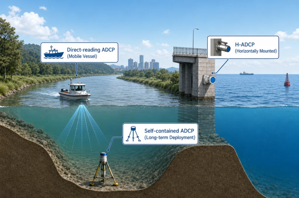
An ADCP that works brilliantly on a research vessel may be completely unusable on a mooring — and vice versa. Deployment mode determines your power source, data recovery path, and physical mounting requirements. Decide this early.
Vessel-Mounted (Direct-Reading)
If your work involves survey transects, repeat sections, or adaptive sampling, a vessel-mounted direct-reading ADCP is the default choice. The instrument sends data up the cable in real time, and you see profiles while steaming. Hull-mounted installations need a sea chest or moon pool; over-the-side mounts are simpler but add drag and require fair-weather operations.
What to check: cable length limits for your chosen communication protocol. RS-232 tops out around 15 m without repeaters; RS-422 gives you more range. Also confirm your acquisition computer can handle the ping rate you want — some older research vessels still run legacy acquisition machines that may bottleneck high-frequency sampling.
Moored (Self-Contained)
Long-term time series — boundary current monitoring, overflow transport estimates, seasonal cycle studies — demand self-contained ADCPs. These instruments run on internal batteries and store data to internal memory. You deploy, walk away, and hope the recovery cruise finds them still recording.
What to check: battery capacity at your target sampling interval. A 75 kHz ADCP pinging every 15 minutes can run 12+ months on a well-designed external battery pack. Crank the ping rate to every 30 seconds and you might not make it to six months. Do the power math before you weld the mooring cage shut.
Bottom-Mounted and Trawl-Resistant
For near-seabed processes — benthic boundary layer dynamics, sediment resuspension, dense overflows — a bottom-mounted ADCP looking upward is the standard approach. Trawl-resistant bottom mounts (TRBMs) protect the instrument in fishing grounds, but they add cost, weight, and deck-handling complexity.
AUV and ROV Integration
Under-ice surveys, deep-scattering-layer tracking, and mine-countermeasure applications increasingly use ADCPs on autonomous or remotely operated vehicles. Here size, weight, and power draw dominate the decision. Phased-array transducers — which pack four beams onto a single flat face — have a natural advantage in these space-constrained applications.
3. Beam Architecture: Piston Transducers vs. Phased Array
For decades, the standard ADCP used four individual piston transducers arranged in a Janus configuration — each pointed 20–30° off vertical, providing the three-dimensional velocity solution. This design is well understood, widely validated, and still the right answer for many applications.
Phased-array ADCPs use a single flat transducer face with multiple elements. By electronically steering the beam, they produce four beams from one aperture. The payoff: a smaller, flatter transducer head that fits into tighter mounts, sheds biofouling more evenly, and can achieve better bottom-tracking performance at lower frequencies.
When the difference matters: If you are mounting an ADCP inside a trawl-resistant bottom mount or on the hull of a small AUV, the phased array’s compact form factor is a genuine advantage. For a large research vessel with a dedicated sea chest, the piston-vs-phased-array distinction is less critical — either will work, and your choice should come down to frequency, range, and accuracy specs rather than transducer geometry.
It is worth noting that at lower frequencies — 75 kHz and below — phased-array designs have become increasingly common because the transducer face for a piston equivalent would be impractically large. This is one reason the 75 kHz band has seen strong innovation in recent years.
4. The Deep-Ocean Sweet Spot: Why 75 kHz Earns Its Place
There is a gap between coastal ADCPs (300–600 kHz, good to ~150 m) and full-ocean-depth systems (38 kHz, good past 1000 m). A 38 kHz transducer head can be 40–50 cm across and weighs enough to need a dedicated winch. A 600 kHz unit might fit in a backpack but cannot see past the mixed layer in blue water. For many oceanographic research scenarios — continental slope moorings, basin-scale surveys that do not need abyssal coverage, shelf-break exchange studies — neither extreme fits.
A 75 kHz ADCP profiles reliably to 500–700 m with cell sizes in the 4–8 m range. That is deep enough to capture the permanent thermocline and the upper intermediate water masses, yet the resolution is fine enough to resolve internal wave shear and near-inertial oscillations — phenomena that coarser 38 kHz bins simply average out.
A Closer Look: Phased-Array 75 kHz ADCPs
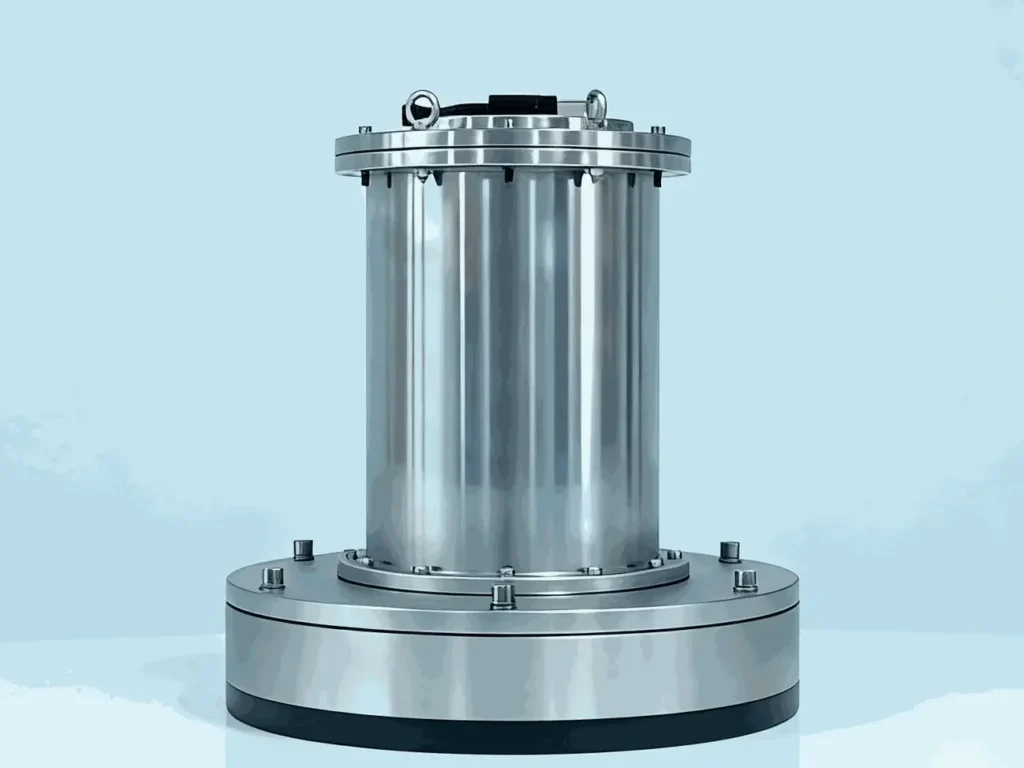
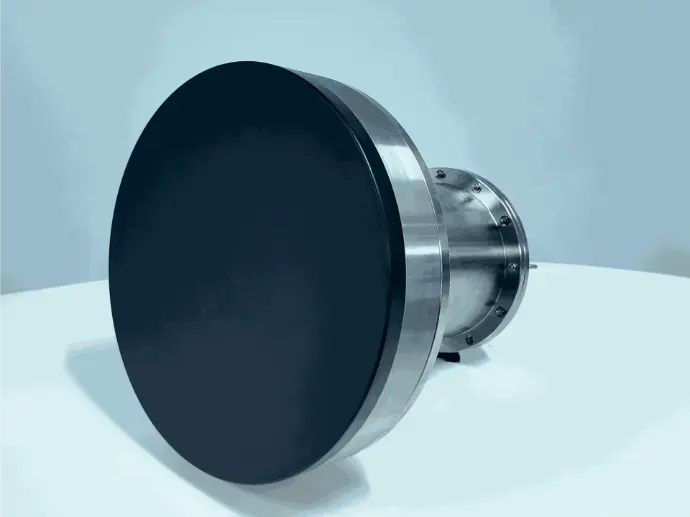
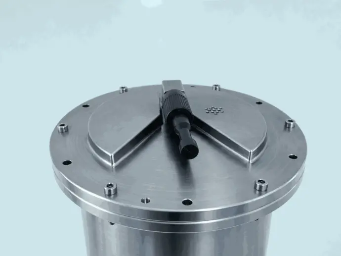
One instrument that exemplifies this class is the Oceantek 75 kHz phased-array ADCP. It uses a flat-face phased-array transducer — significantly more compact than a piston 75 kHz would be — and delivers the kind of velocity accuracy (typically ±0.5% of water velocity or better) that peer reviewers expect from a research-grade instrument.
What makes the Oceantek 75k ADCP worth a look for oceanographic users is the combination of broadband signaling for precision and the phased array’s robust bottom-tracking performance. If your work involves measuring absolute transport across a section — where you need both water-column profiles and a solid bottom-track reference — this matters. The instrument is available in both direct-reading (for vessel surveys) and self-contained (for mooring deployments) configurations, so the same transducer technology can serve across both modes of a research program.
For a concrete scenario: imagine a mooring at 600 m on the continental slope off the Iberian margin, measuring Mediterranean Outflow Water. A 150 kHz ADCP would not reach the core of the outflow at 600–800 m. A 38 kHz would reach it but resolve the vertical structure with bins of 16–24 m — and the Meddy cores you care about might only be 50–80 m thick. A 75 kHz instrument operating with 8-m bins captures that structure while reaching the target depth. That is the kind of match that repays the effort of careful instrument selection.
5. Specifications That Actually Show Up in Your Data
Spec sheets can be overwhelming. Focus on the handful of parameters that directly affect whether your data passes quality control.
Velocity Accuracy and Ping Strategies
A quoted accuracy of “±0.5% of water velocity ±0.5 cm/s” is typical for research-grade ADCPs. But that number assumes a certain number of pings averaged together — often 300 or more. If your vessel is steaming at 10 knots and you want one ensemble every 60 seconds, check that your ping rate and averaging strategy can deliver the stated accuracy under your actual operating conditions. Broadband (coded-pulse) processing improves the single-ping standard deviation substantially; narrowband is simpler but noisier at the same ping count.
Cell Size Flexibility
Most ADCPs let you configure cell size in software — but only within a range that the transducer frequency and bandwidth support. A 75 kHz instrument might offer cells from 2 m to 16 m. Smaller cells give finer vertical detail but fewer of them before the signal fades into noise. Larger cells extend range at the cost of vertical resolution. Being able to adjust this in the field, based on actual water-column conditions, is valuable. Look for instruments that allow cell-size changes without firmware reconfiguration.
Bottom Tracking
Bottom tracking provides the absolute velocity reference — without it, your profiles are relative to the moving platform and you need external navigation (GPS, LADCP workflow) to close the reference frame. A good bottom-tracking ADCP holds lock on the seabed across a range of bottom types — mud, sand, gravel, rock — and gives you a “percent good” metric so you can flag ensembles where bottom lock was marginal.
Phased-array transducers tend to have an edge here: the flat face and wider acoustic footprint produce a stronger bottom return at low frequencies. If your research involves sections that cross from soft sediment to hard rock, bottom-tracking robustness should be high on your spec-sheet checklist.
Integrated Sensors
Every ADCP ships with a pressure sensor, temperature thermistor, tilt sensor, and compass. The questions are accuracy and calibration stability. A pressure sensor that drifts 0.5 dbar over a 12-month mooring deployment introduces a depth error in every bin. A compass that is not properly calibrated for the instrument’s magnetic environment (steel mooring cage, nearby batteries) produces velocity vectors rotated by an unknown angle. For mooring work, budget for a pre-deployment compass calibration — and prefer instruments where the calibration procedure is well documented and repeatable in the field.
6. Field Realities: Power, Biofouling, and Data Logistics
Spec sheets describe a lab instrument. Field deployments describe reality. The gap between the two is where data is won or lost.
Power Budgeting
For a moored self-contained ADCP, the power budget is the deployment’s single point of failure. A typical 75 kHz phased-array ADCP draws roughly 2–4 W when pinging at a moderate ensemble interval — but confirm this against the actual configuration you plan to use. External battery packs (alkaline or lithium) add cost and weight; lithium packs last longer but come with shipping and handling restrictions. Build your power budget around the worst-case cold-water scenario: batteries deliver less capacity at 2°C than at 20°C, and deep moorings are cold moorings.
Biofouling
In productive waters, a transducer face can foul within weeks. Biofouling attenuates the acoustic signal unevenly across beams, producing biased velocity estimates. Phased-array faces, being flat and continuous, are somewhat easier to protect with anti-fouling coatings and shed growth more uniformly than individual piston heads. No transducer is immune, but the flat geometry simplifies your anti-fouling strategy.
Data Storage and Telemetry
A self-contained ADCP recording at 1 Hz fills internal memory faster than many researchers expect. A 16 GB card sounds generous until you calculate that 12 months of 1-Hz ensembles (with four beams, 100 bins each) can approach or exceed that. Check whether your instrument supports removable storage or inductive modem offload — recovering a mooring and finding the memory full after month three is an avoidable heartbreak. Some modern instruments support real-time telemetry via acoustic modem or inductive link to a surface buoy with satellite backhaul, so you can monitor data quality — and battery voltage — during the deployment.
7. Software, Data Formats, and Integration with Your Processing Chain
An ADCP produces binary data files — typically in Teledyne RDI’s PD0 format, which has become the de facto standard — plus manufacturer-specific raw formats. Before purchasing, confirm what formats the instrument exports and whether your processing pipeline can read them natively.
If your lab runs CODAS (the University of Hawaii’s Common Ocean Data Access System), you need PD0 or compatible binary output. If you work in Python, the pyADCP and xarray libraries read PD0 and NetCDF with reasonable fidelity. If your workflow is MATLAB-based, check that the manufacturer provides a reader toolbox — or that the community has written one.
Time synchronization is the integration headache nobody talks about until data from the ADCP, CTD rosette, and shipboard GPS disagree by 2–3 seconds and the resulting shear estimates look suspect. Look for instruments that accept a PPS (pulse-per-second) input from a GPS receiver — this keeps the ADCP clock aligned with the ship’s navigation data to within milliseconds, not seconds.
8. Budget Realism: Purchase Price Is the Start, Not the End
ADCP prices scale with depth capability and transducer complexity. A 600 kHz river ADCP might cost $15,000–$25,000. A research-grade 75 kHz phased-array ADCP runs higher — typically $40,000–$70,000 depending on configuration — and a full 38 kHz deep-ocean system can exceed $100,000 with accessories. These are rough brackets; exact pricing depends on cabling, pressure housings, battery packs, and any custom mounting hardware.
The bigger line items after purchase:
- External battery packs — lithium packs for a 12-month mooring deployment can cost $3,000–$8,000 depending on capacity.
- Mounting cages and acoustic releases — a deep-water acoustic release alone is $5,000–$15,000.
- Cables and deck units — research-vessel-grade armored cable with proper terminations is not cheap, and deck units for direct-reading systems add several thousand dollars.
- Calibration — budget for a pre- and post-deployment compass calibration at minimum; some labs also request tank calibrations for velocity validation.
- Spares — O-rings, dummy plugs, desiccant packs, and a spare cable are the cheapest insurance you will ever buy.
Warranty terms and manufacturer support responsiveness matter more than a 5% price difference between competing instruments. An ADCP that ships with a three-year warranty and has an engineer who answers email within 24 hours is worth more than a marginally cheaper unit supported by a ticket system that takes a week. Ask colleagues what their post-sale experience has been — this is a small community, and reputations are earned in the field.
9. Decision Checklist: A One-Page Summary
Work through these questions in order. By the time you answer the last one, your shortlist should be very short.
- What is the deepest feature you need to profile? This gives you the minimum frequency. Add 20–30% depth margin for real-world conditions (suspended sediment, lower backscatter).
- What platform are you using? Vessel → direct-reading. Mooring → self-contained. AUV/ROV → compact form factor, likely phased-array.
- How fine must your vertical resolution be? If your features are O(10 m) thick, you need cells no larger than 4–8 m. If bin size at your required frequency is too coarse, consider whether you can move up one frequency band and still reach your target depth.
- Do you need absolute velocity? If yes, bottom tracking is essential. Vessel surveys also need GPS synchronization.
- What is your deployment duration? Confirm battery capacity and memory at your planned sampling rate. Add 30% margin.
- What data format does your processing chain expect? PD0 is the safest default. Confirm export options.
- What is your total budget — including accessories, spares, and calibration? The instrument itself is typically 60–70% of the total initial outlay.
10. Frequently Asked Questions
What frequency ADCP do I need for 1000-meter water depth?
You need a 38 kHz ADCP to profile reliably to 1000 m. A 75 kHz instrument will typically reach 500–700 m under good conditions but will lose bottom return before 1000 m. If your science target is at 800–1000 m, 38 kHz is the right band — even though cell sizes will be coarse (12–24 m).
Can one ADCP handle both vessel-mounted surveys and long-term moorings?
Yes — if you choose an instrument available in both direct-reading and self-contained configurations. The Oceantek 75k ADCP is an example: the same transducer and electronics platform ships in a direct-reading housing for real-time vessel surveys, and a self-contained housing for autonomous mooring deployments. This means your calibration methodology, data format, and processing scripts stay consistent across both modes.
What is the difference between a DVL and an ADCP?
A Doppler Velocity Log (DVL) is optimized for bottom-tracking navigation — it prioritizes bottom lock, low latency, and compact form factor for AUV/ROV use. An ADCP is optimized for water-column current profiling — it prioritizes range resolution, velocity accuracy, and multi-layered water tracking. Some instruments blur the line (a DVL can profile water currents, and an ADCP can bottom-track), but if your primary goal is oceanographic current measurement, buy an ADCP, not a DVL.
How often does an ADCP need recalibration?
Compass calibration should be done before every deployment — ideally with the instrument mounted in its deployment cage. Velocity calibration (transducer geometry) is stable for years on piston-based designs; phased-array instruments are similarly stable but fewer long-term drift studies exist simply because the technology is newer. A tank calibration every 2–3 years is reasonable for a research instrument in active use.
Is a phased-array ADCP worth the extra cost for shelf-sea work?
For shelf-sea research (50–200 m), a 150 kHz or 300 kHz piston ADCP will do the job well, and phased-array advantages in form factor and bottom tracking are less critical at these ranges. The extra cost of a phased-array 75 kHz instrument makes most sense when you need the depth capability — shelf-break, slope, and blue-water work below 200 m — and can benefit from the smaller transducer footprint.
Still Unsure? Talk to an Applications Engineer
Every research program has constraints that a general article cannot anticipate — a specific winch cable length, a mooring design already approved, a budget fixed in a grant proposal written two years ago. If you would like to discuss your specific scenario with someone who works on ADCPs daily, the team at Oceantek includes applications engineers who have deployed instruments in most of the world’s ocean basins. They can help you narrow the shortlist to the one or two instruments that actually fit.