📊 Executive Summary
Flood frequency and intensity are rising globally — and the difference between a flood event and a flood disaster often comes down to minutes of warning lead time. An ADCP-based real-time river monitoring network closes the gap between “we saw the rain” and “we know the discharge,” providing the continuous, quantitative flow data that hydrological models and emergency managers need to issue timely, location-specific warnings.
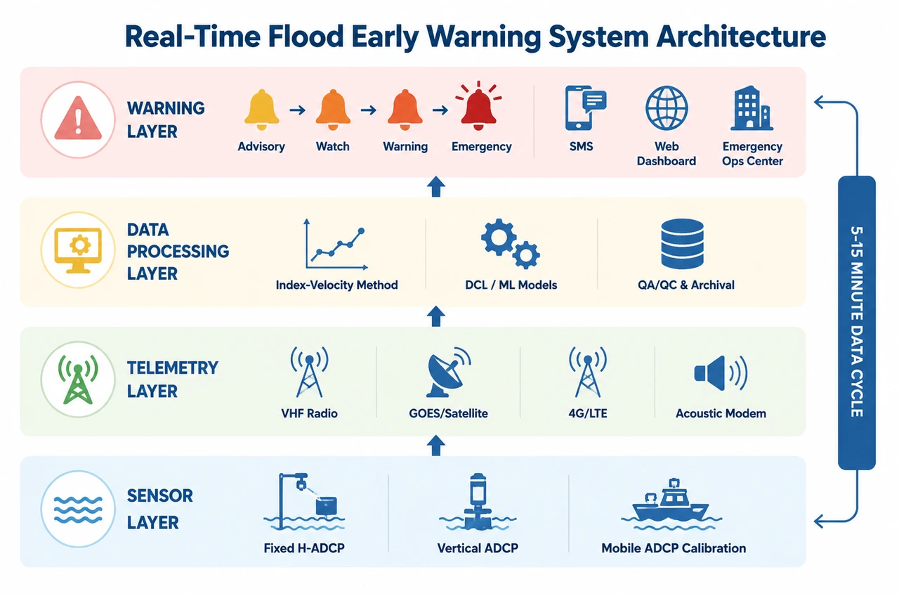
This guide covers the end-to-end architecture of an ADCP flood early warning system — from fixed H-ADCP sensors on the riverbank and telemetry design through to data processing algorithms, multi-threshold alert logic, and dissemination — with equipment selection matrices, WMO/USGS regulatory alignment, and four operational case studies from Charlotte (USA), the Edogawa River (Japan), the Haihe Basin (China), and the Neelum Valley (Pakistan).
📑 Table of Contents
- Introduction: The Architecture Gap in Flood Early Warning
- The Sensor Layer: Choosing the Right ADCP Configuration
- The Telemetry Layer: Getting Data Out in Real Time
- The Data Processing Layer: From Raw Velocity to Actionable Discharge
- The Warning Layer: Thresholds, Alerts, and Dissemination
- Case Studies: Four Architectures in Practice
- Equipment Selection for Flood Warning Networks
- Implementation Roadmap
- Frequently Asked Questions
- Conclusion
1. Introduction: The Architecture Gap in Flood Early Warning
A flood early warning system is only as strong as its weakest data link. The typical failure mode is not a lack of rainfall data — weather radar and satellite precipitation estimates have improved dramatically. The failure mode is not knowing what the water is actually doing in the river channel.
Three gaps create this blind spot:
- The temporal gap: Manual discharge measurements — sending a crew to the river with a current meter or moving-boat ADCP — capture a snapshot. But flood discharge can double in hours. If your measurement interval is weekly and the flood peaks on Tuesday, you missed it. The WMO’s end-to-end early warning system (E2E EWS) framework explicitly requires continuous real-time monitoring and surveillance as the second operational phase, alongside forecasting (WMO Technical Regulations Vol. III — Hydrology).
- The spatial gap: Rainfall-runoff models need upstream boundary conditions. Without real-time discharge data at key tributary confluences and main-channel control points, models propagate errors downstream. A 2025 framework in Nature Water (Oh & Bartos) demonstrated that data-driven gauge network optimization — selecting monitoring sites that best capture the spatiotemporal structure of a basin — significantly outperforms uniform or population-based placement for reconstructing streamflow at ungauged locations.
- The hysteresis gap: The traditional stage-discharge rating curve assumes a one-to-one relationship between water level and flow. During floods, this assumption breaks down catastrophically. The same water level on the rising limb of the hydrograph can correspond to a discharge 30–40% higher than on the falling limb — because the flood wave’s unsteady momentum adds velocity that the stage measurement alone cannot see (Muste & Kim, MDPI Water, 2022). An H-ADCP measuring index velocity captures this kinematic signature directly.
An ADCP-based real-time monitoring network addresses all three gaps simultaneously: continuous temporal coverage, spatial coverage through a network of fixed and mobile stations, and kinematic accuracy through direct velocity measurement. The question is not whether to use ADCPs for flood warning — it is how to design the architecture so the system works when it matters most.
2. The Sensor Layer: Choosing the Right ADCP Configuration
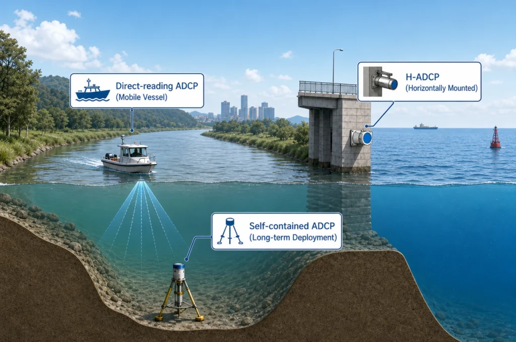
The sensor layer is where flood data originates. A well-designed flood warning network uses three ADCP deployment configurations working together — no single instrument type covers all monitoring objectives.
2.1 H-ADCP: Fixed Horizontal Monitoring — the Backbone
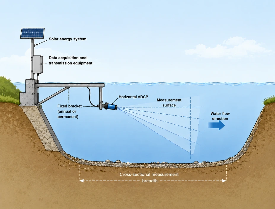
The Horizontal ADCP (H-ADCP) is the workhorse of any real-time flood warning network. Mounted permanently on a riverbank, bridge pier, or channel wall, it measures a horizontal velocity profile across the channel 24 hours a day, 365 days a year with no operator on site. The Oceantek HADCP-600 uses three acoustic beams — two horizontal beams at ±20° for cross-channel velocity profiling and a vertical reference beam — to cover up to 90 m horizontal range with ±0.3% ±3 mm/s accuracy at a 2 Hz data refresh rate. Data output is via RS-232/RS-422 serial interface, connecting to an external datalogger with cellular or satellite telemetry for real-time transmission.
The H-ADCP’s key operational advantage for flood warning is continuity through the event. Unlike mobile survey crews — who cannot safely deploy during peak flood conditions — the H-ADCP captures the entire hydrograph: rising limb, peak, and recession. This continuous time series is the input both for real-time threshold alerting and for post-event calibration of hydrological models.
2.2 Vertical ADCP: Fixed Bottom-Mounted Profiling
Where the monitoring objective requires vertical velocity structure — for example, at a reservoir outflow or a deep channel section where stratified flow may develop during floods — a bottom-mounted vertical ADCP provides the depth-resolved data that a horizontal instrument cannot. Deployed on the riverbed in a trawl-resistant mount, the instrument profiles the full water column in user-defined depth cells (1–255 cells, configurable cell size), transmitting data through a cabled connection to a shore-based datalogger or a surface buoy with telemetry.
This configuration is especially valuable at dam and reservoir outlets — where gate operations during flood release create complex, depth-dependent velocity fields — and at tidal river reaches where bidirectional flow and salinity stratification require full water-column resolution to compute net discharge accurately. Vertical ADCPs in self-contained configuration with 64 GB internal storage and external battery packs can operate autonomously for months, making them suitable for remote locations where maintenance access is seasonal.
2.3 Moving-Boat ADCP: Periodic Calibration and Flood Peak Surveys
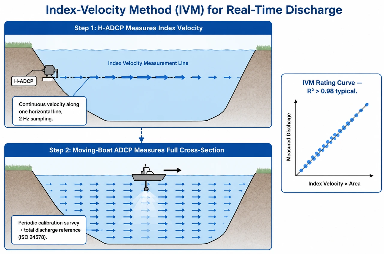
Fixed H-ADCPs measure index velocity along a single horizontal line — not total cross-sectional discharge. To convert index velocity to discharge, the H-ADCP must be calibrated against reference measurements that cover the full cross-section. This is where the moving-boat ADCP enters the architecture.
The River-ADCP-600-FA5 is purpose-built for this role. With 5 beams — four piston transducers in Janus arrangement (20° beam angle) plus a dedicated vertical piston beam for simultaneous bathymetry — it profiles 0.5–65 m depth range at ±0.25% ±2 mm/s accuracy with integrated GPS (no external antenna required). Its 4 Hz maximum sampling rate (1–2 Hz for cross-section work) and 0.5–110 m bottom-tracking range make it effective in the turbid, high-sediment conditions typical of flood flows. The calibration protocol follows ISO 24578:2021 methodology and USGS Techniques and Methods 3-A8: a minimum of four transects (two in each direction), compass calibration before each survey day with error <0.5°, and a moving-bed test to verify bottom-track validity.
During a flood event, the moving-boat ADCP serves a second critical function: flood peak discharge verification. As waters recede and conditions allow safe navigation, the survey crew can measure the peak discharge directly — providing the definitive data point for rating curve extrapolation and flood frequency analysis.
2.4 Multi-Angle Deployment: Redundancy and Accuracy
Single-instrument deployments have a single point of failure. A 2024 study in the Yangtze basin (published via DOAJ) demonstrated that dual-H-ADCP, multi-angle deployments — where two instruments with different frequencies (e.g., 600 kHz and 300 kHz) are installed at varying tilt angles along the same cross-section — significantly improve monitoring robustness. At Zhicheng Station, dual-device configurations achieved R² of 0.9903 for index-velocity-to-discharge correlation, with relative runoff volume errors of −0.36% to 1.25%.
The multi-angle approach addresses three operational challenges simultaneously:
- Backwater effects: When downstream water levels rise (from a tributary flood or tidal influence), a single horizontal measurement line may no longer represent the full cross-section. A second instrument at a different angle or vertical position captures the altered flow structure.
- Turbidity attenuation: During extreme floods, suspended sediment concentrations can exceed 10–20 g/L, attenuating the acoustic signal and reducing the H-ADCP’s effective range. A lower-frequency companion instrument (300 kHz) penetrates further in high-concentration flows.
- Instrument redundancy: If one H-ADCP fails — due to debris impact, power loss, or fouling — the second instrument maintains the data stream. For public-safety-critical stations, this redundancy is not optional; the EGU 2025 NFFWS guidelines explicitly recommend backup instrumentation for priority gauges (Roberts et al., Met Éireann).
2.5 Sensor Layer Selection Matrix
| Monitoring Objective | Deployment | Key Instrument | Data Output | Role in EWS |
|---|---|---|---|---|
| Continuous cross-channel velocity profile | Fixed bank/bridge mount | HADCP-600 (3-beam, 600 kHz, 90 m range) | Index velocity at 2 Hz → 5–15 min averaged discharge via IVM | Primary: Real-time threshold monitoring + data feed to forecast models |
| Vertical velocity structure (reservoir outlet / deep channel) | Fixed bottom mount | Ocean-ADCP-300-FA4 / Ocean-ADCP-600-FA4 (4-beam Janus) | Full water-column velocity profile, configurable cell size | Supplementary: Stratified flow detection during reservoir flood release |
| Periodic H-ADCP calibration + flood peak surveys | Mobile (manned boat or USV) | River-ADCP-600-FA5 (5-beam, 600 kHz, integrated GPS) | Full cross-section discharge (ISO 24578 method), simultaneous bathymetry | Calibration + Verification: Pre/post-flood season calibration; post-event peak verification |
| Emergency flood survey (hazardous conditions) | USV (unmanned) | River-ADCP-M9 (9-beam dual-frequency, 1 MHz/3 MHz + 500 kHz vertical) | Discharge + bathymetry in a single autonomous pass | Emergency: Deployable when crew safety prevents manned surveys |
3. The Telemetry Layer: Getting Data Out in Real Time
The most accurate ADCP in the world is useless for flood warning if its data stays inside the instrument. The telemetry layer is what transforms a local velocity measurement into a networked, actionable data stream reaching emergency managers and forecast models within minutes.
3.1 Communication Options Matrix
| Technology | Range | Latency | Power Draw | Best For | Operational Example |
|---|---|---|---|---|---|
| VHF/UHF Radio | Line-of-sight (~15–30 km per hop) | <1 min | Low | Regional networks with repeater infrastructure; flood-proof (no ground infrastructure to fail) | USGS FINS Charlotte — 52 streamgages + 72 raingages using ALERT protocol over VHF |
| 4G/LTE Cellular | Network coverage dependent | <30 s | Low–Medium | Stations with reliable cellular coverage; lowest deployment cost | Nakdong River, Korea — ADSL primary + CDMA secondary, VPN-secured |
| GOES Satellite | Continental (requires clear sky to satellite) | 5–15 min (scheduled transmission windows) | Medium | Remote stations without ground infrastructure; USGS standard for backcountry gauges | USGS streamgages across continental USA — standard DCP (Data Collection Platform) configuration |
| Iridium/Inmarsat Satellite | Global | <1 min | Medium–High | Remote basins without any ground infrastructure — essential for Himalayan, Andean, Arctic deployments | Neelum Basin, Pakistan — hybrid satellite + GSM, cloud platform aggregation |
| Underwater Acoustic Modem | 1–5 km underwater | <1 min | Low (acoustic) / Medium (surface buoy) | Cable-free underwater-to-surface link; pairs with surface LTE buoy | EvoLogics Northern Germany — riverbed ADCP → acoustic modem → surface buoy → LTE → shore |
3.2 Power and Resilience Design
Floods destroy infrastructure. The telemetry system must survive the event it is monitoring. Three design principles apply:
- Autonomous power: Solar panel + battery is the standard configuration. The HADCP-600’s low power consumption (10–26 V input) pairs with a 50–100 W solar panel and deep-cycle battery bank sized for 5–7 days of autonomy — sufficient to ride through the extended cloud cover that accompanies flood-producing storms. The USGS Indiana network study (Glatfelter & Butch, 1994) specifically recommends solar-powered stations with satellite transmitters for remote flood monitoring.
- Local data storage: 64 GB onboard Micro SD storage in every Oceantek ADCP ensures that even if the telemetry link fails during the storm peak, no data is lost. When the link is restored, the backlog transmits automatically. This “store-and-forward” architecture is standard in the EvoLogics German river network and proved critical during the July 2025 Haihe flood when communication infrastructure itself was damaged — the ADCPs had recorded 220,000+ situation records locally.
- Dual-path telemetry: A primary channel (cellular or radio) with automatic failover to a backup channel (satellite) eliminates the single-point-of-failure risk. The USGS FINS network achieves this through VHF radio primary with GOES satellite backup; the Neelum Basin system in Pakistan uses GSM primary with satellite failover. The additional hardware cost is a fraction of the cost of missing a flood peak due to a communication outage.
4. The Data Processing Layer: From Raw Velocity to Actionable Discharge
An H-ADCP measures line velocity — typically along 1–255 cells across a single horizontal profile. Converting this to total cross-sectional discharge in real time is the central algorithmic challenge of the data processing layer.
4.1 The Index-Velocity Method (Standard Approach)
The index-velocity method (IVM) is the operational standard used by the USGS, hydrological agencies worldwide, and implemented in H-ADCP real-time monitoring best practices. The workflow:
- The H-ADCP measures a representative “index velocity” — typically the horizontally averaged velocity across a selected subset of cells in the main channel, chosen to maximize correlation with cross-sectional mean velocity.
- Periodic moving-boat ADCP calibration surveys measure the true total discharge across the full cross-section using the ISO 24578 methodology.
- A regression model — typically linear (discharge = a × index velocity × area + b) or power-law — relates the index velocity and stage (which determines cross-sectional area) to total discharge.
- The model is applied to the continuous H-ADCP data stream, producing real-time discharge at the same 5–15 minute reporting interval as the input data.
The IVM’s fundamental advantage over the traditional stage-discharge rating is that it adds a kinematic variable. A stage-only rating sees “water level = 3.2 m” and returns one discharge. An IVM sees “water level = 3.2 m AND index velocity = 1.8 m/s on the rising limb vs. 1.3 m/s on the falling limb” and returns two different, correct discharges. Research by Muste & Kim (MDPI Water, 2022) at USGS index-velocity station #05558300 confirmed that the IVM captures the hysteretic loop structure of flood waves that stage-discharge ratings entirely miss.
4.2 Advanced: Machine Learning Models for Complex Sites
At sites with compound channels, backwater effects, tidal influence, or highly unsteady flow, linear index-velocity models may struggle. A 2024 Deep Characteristic Learning (DCL) model published in ScienceDirect addressed this by:
- Using Principal Component Analysis (PCA) to reduce 128 H-ADCP velocity cells to a manageable feature set.
- Running six machine learning models in parallel — BP neural network, Elman neural network, RBF network, GRNN, SVM, and multiple linear regression (MLR) — each mapping reduced velocity features to total discharge.
- Applying a Genetic Algorithm–Particle Swarm Optimization (GA-PSO) hybrid for automatic feature selection and model hyperparameter tuning.
At Luohu Station — a tidally influenced, backwater-affected site on the Yangtze system — the DCL approach achieved RMSE of 6.06 m³/s and R² of 0.93 over a three-year test period, demonstrating strong self-learning capability even with limited training samples. For sites where conventional IVM calibration produces unacceptable uncertainty, machine learning models running on the central processing server offer a pathway to operational accuracy.
4.3 Data Processing Architecture
Regardless of the algorithm choice, the processing architecture follows a consistent pattern:
| Stage | Location | Function |
|---|---|---|
| Edge pre-processing | On-site datalogger | Time-averaging (1–2 Hz raw → 5–15 min blocks), basic quality flags (SNR, percent-good, error velocity), data compression, store-and-forward buffering |
| Central processing | Cloud or agency server | IVM/DCL discharge computation, cross-station data fusion, rating curve application, QA/QC with automated outlier detection, archival to hydrological database |
| Forecast ingestion | Hydrological model interface | API-based discharge data feed to HEC-RAS, SWAT, HEC-HMS, or custom forecast models at the model’s native time step; model output returned for comparison against measured data |
| Visualization | Web dashboard | Real-time hydrograph display with threshold overlays; multi-station comparison; historical reference curves; automated report generation (daily, event, annual) |
5. The Warning Layer: Thresholds, Alerts, and Dissemination
The warning layer is where data becomes decision. A well-designed alert framework has three components: what triggers the alert, who receives it, and what they are supposed to do.
5.1 Multi-Threshold Graded Alert Design
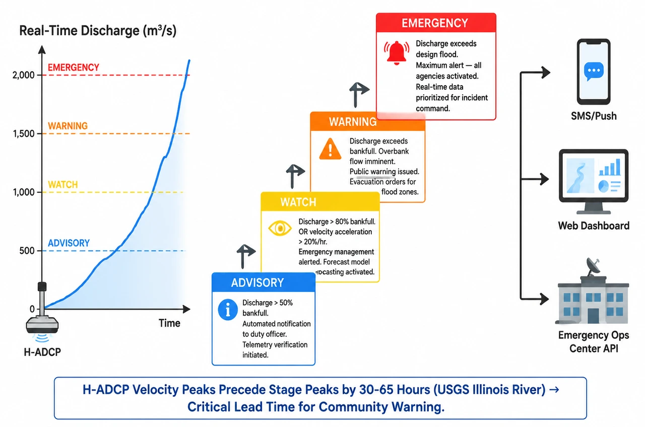
The WMO recommends a graded warning structure that escalates as conditions deteriorate. For a discharge-based ADCP early warning system, a four-tier framework maps naturally to the hydrograph:
| Alert Level | Trigger Condition | Example Threshold | Action |
|---|---|---|---|
| Advisory (Blue) | Discharge exceeds 50% of bankfull | Pre-flood season baseline + 50% | Automated notification to hydrology duty officer; begin 15-min data logging; verify telemetry link to all upstream stations |
| Watch (Yellow) | Discharge exceeds 80% of bankfull OR rate of rise exceeds threshold | Stage rising >0.3 m/hr sustained for 2+ hours; index velocity acceleration >20% per hour | Alert to emergency management agency; activate forecast model now-casting; prepare field crew for mobile calibration survey |
| Warning (Orange) | Discharge exceeds bankfull; overbank flow imminent or occurring | Bankfull discharge (site-specific, from channel survey) | Public warning issued; evacuation orders for flood-prone zones; field crew deployed for peak discharge verification if safe |
| Emergency (Red) | Discharge exceeds design flood (e.g., 100-year event) OR critical infrastructure at risk | Design flood discharge; bridge scour threshold; levee overtopping level | Maximum alert: all agencies activated; evacuation in progress; real-time data feed prioritized for incident command |
5.2 Alert Dissemination Channels
Alert data must reach decision-makers through multiple redundant channels. The Panchganga River IoT flood warning system in India demonstrates a multi-channel approach: SMS and email to registered stakeholders, push notifications via a mobile application, API endpoints for integration with government emergency dispatch systems, and a public-facing web dashboard with real-time hydrograph visualization and color-coded station status. The USGS FINS network adds a dedicated radio channel for direct communication with emergency operations centers — independent of public communication infrastructure.
5.3 The Velocity-Peak-Before-Stage-Peak Advantage
Perhaps the most operationally significant finding in H-ADCP flood warning research comes from six years of data at USGS station #05558300 (Illinois River at Henry, Illinois). Analysis of flood hydrographs revealed a consistent pattern: index-velocity peaks precede stage (water level) peaks by 30–65 hours — that is, 1.25 to 2.7 days (USGS Patent 20230281493, 2023).
This time lag has profound implications for warning system design. By monitoring the H-ADCP velocity data stream in real time and detecting the velocity peak as it occurs, the system can forecast the stage crest magnitude and arrival time using directly measured velocity and stage data alone — without running a rainfall-runoff model, without a rating curve, and without waiting for upstream gauge data. Hindcasts for the largest storms of 2014–2019 predicted stage crest magnitudes within ~10% (most within ~5%).
6. Case Studies: Four Architectures in Practice
6.1 USGS FINS — Charlotte/Mecklenburg County, North Carolina, USA
Architecture: 52 streamgages + 72 raingages → VHF radio (ALERT protocol) + GOES satellite backup → USGS National Water Information System (NWIS) → multi-agency emergency operations center.
Evolution: Developed after the catastrophic floods of August 1995 and July 1997, the FINS network evolved over 30 years from a landline-and-satellite system to a true real-time dual-path system. Most stations transmit at 5-minute intervals under normal conditions; when site-specific thresholds are exceeded during storm events, immediate event-triggered reporting pushes stream level and rainfall data to emergency managers within seconds.
Key design principle: The ALERT protocol is event-driven and non-continuous; regular-interval data are loaded into NWIS for the permanent historical record. This dual architecture provides both immediate emergency response data and long-term continuous datasets for flood frequency analysis, climate trend detection, and model calibration.
Data source: USGS Flood Information and Notification System (FINS), updated December 2021.
6.2 Edogawa River, Japan — H-ADCP + DIEX Numerical Simulation
Architecture: 600 kHz H-ADCP fixed in compound channel → real-time data feed → DIEX (Dynamic Interpolation and EXtrapolation) data-assimilation model → discharge with ~5.0% RMSE, outperforming conventional IVM (~12.0%) during large floods.
Why it matters: The Edogawa case demonstrates that in compound channels — where a deep main channel and shallow floodplain coexist — the conventional index-velocity method breaks down because a single horizontal measurement line cannot capture the velocity contrast between the fast main-channel flow and the slow floodplain flow. Coupling the H-ADCP with a numerical simulation that dynamically interpolates and extrapolates across the full compound section closes this accuracy gap.
Data source: Elsevier Pure / MLIT Japan combined H-ADCP and numerical simulation system.
6.3 Haihe River Basin, China — Digital Twin Architecture
Architecture: Multi-sensor network (ADCP + radar level + rain gauge + GNSS deformation) → central processing → 3D digital twin platform → automated alarm engine with 96.2% accuracy.
July 2025 flood performance: During a major flood event in July 2025, the system processed over 220,000 situation records. The automated alarm engine achieved 96.2% accuracy. The digital twin reduced mean time-to-detect from hours to seconds and mean time-to-repair from 4 hours to 1 hour — metrics that translate directly to lives protected and infrastructure saved.
Data source: CNKI / Water Resources and Hydropower Engineering (2026).
6.4 Neelum Basin, Pakistan — Remote Himalayan Deployment
Architecture: 4 real-time streamflow stations (ADCP + non-contact radar level) → hybrid satellite + GSM telemetry → cloud-based hydromet platform → inflow forecasting for Neelum Jhelum Hydropower Plant + flash-flood warning for downstream communities.
The extreme-environment challenge: The Neelum Valley in Azad Kashmir is a high-altitude Himalayan basin with no grid power, no GSM coverage at most station locations, and access roads that close for months each winter. The monitoring network was designed from the ground up for these constraints: solar-only power with multi-day battery autonomy, satellite as primary telemetry with GSM backup where coverage exists, and non-contact sensing (radar level + ADCP) to minimize debris-damage risk during monsoon-season flash floods.
Data source: CDigital case study / WAPDA Neelum Jhelum Hydropower Plant monitoring network.
7. Equipment Selection for Flood Warning Networks
The equipment selection matrix below maps monitoring objectives to specific instrument configurations, with a focus on the characteristics that matter most in a flood warning context: continuous unattended operation, data refresh rate, communication interface, and robustness under extreme conditions.
| Station Type | Primary Instrument | Key Specs for Flood EWS | Telemetry Interface | Power |
|---|---|---|---|---|
| Fixed H-ADCP (primary monitoring) | HADCP-600 | 3-beam, 600 kHz, 90 m cross-channel, 2 Hz, ±0.3% ±3 mm/s | RS-232/RS-422 → external cellular/satellite modem | 10–26 V, solar + battery |
| Vertical bottom-mount (reservoir outlet / deep channel) | Ocean-ADCP-600-FA4 | 4-beam Janus, 600 kHz, 55–70 m profile, 1–255 cells, 64 GB storage | RS-232/RS-422 | ≤10 W, solar + battery or mains |
| Mobile calibration (periodic survey) | River-ADCP-600-FA5 | 5-beam (4 Janus + 1 vertical), 600 kHz, integrated GPS, 4 Hz max, 0.5–110 m bottom track, ≤3.5 kg | RS-232/RS-422 (direct to survey laptop) | 10–26 V, ≤5 W — vessel battery |
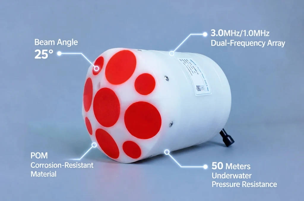
| USV emergency survey | River-ADCP-M9 | 9-beam dual-frequency (1 MHz/3 MHz + 500 kHz vertical), 0.06–40 m profile, 80 m bathymetry, ≤1.5 kg | RS-232/RS-422 via USV telemetry | USV-integrated |
| Stage sensor (companion to H-ADCP) | Radar / bubbler / pressure transducer | Non-contact preferred (debris risk during floods); 1 cm accuracy; 1–5 min reporting | Same datalogger as H-ADCP | Shared with H-ADCP |
All Oceantek ADCPs are manufactured under ISO 9001:2015 certified quality management and output industry-standard PD0 format data compatible with USGS QRev, WinRiver II, and VMT processing software — ensuring that flood discharge data can be reviewed, quality-controlled, and archived using the same tools and workflows already deployed at national hydrological agencies.
8. Implementation Roadmap: 6 Steps to an Operational Flood Warning Network
| Phase | Duration | Key Activities | Deliverable |
|---|---|---|---|
| 1. Risk Assessment | 1–2 months | Identify flood-prone reaches; map vulnerable populations and critical infrastructure; determine required warning lead time (basin response time minus evacuation time); consult historical flood records and rainfall frequency analysis | Flood risk map with lead-time requirements per reach |
| 2. Site Selection | 1 month | Apply gauge network optimization framework (EGU 2025 / Nature Water 2025 methodology); select H-ADCP mounting locations with stable banks, representative cross-sections, and telemetry line-of-sight or cellular coverage; designate priority stations for redundancy | Station siting report with coordinates, access plan, and telemetry feasibility |
| 3. Instrumentation | 1–2 months | Install H-ADCP mounting brackets, stage sensor, datalogger, solar power system, and telemetry modem; configure data averaging intervals and alert thresholds; conduct initial moving-boat calibration survey (≥4 transects, ISO 24578 compliant) | Commissioned stations with baseline IVM calibration curves |
| 4. Telemetry Integration | 1 month | Establish primary and backup communication paths; configure data formats and transmission protocols; implement store-and-forward buffer; test under simulated communication-failure conditions | End-to-end data flow verified from sensor to central server |
| 5. Calibration and Verification | Ongoing | Pre-flood season calibration survey (all stations); verify index-velocity rating curves; conduct moving-bed tests; recalibrate after any channel-altering flood event; annual sensor intercomparison | Validated rating curves; calibration documentation for regulatory audit |
| 6. Operation and Maintenance | Continuous | Monthly visual inspection of mounting hardware, cables, and solar panels; annual comprehensive inspection (simulated alert test, instrument diagnostic check, battery replacement if needed); pre-flood season preventive maintenance on all stations | Maintenance logs; annual network performance report |
9. Frequently Asked Questions
Q: What is an H-ADCP and how does it work in flood warning systems?
An H-ADCP (Horizontal Acoustic Doppler Current Profiler) is a fixed, side-looking instrument mounted on a riverbank, bridge pier, or channel wall that measures horizontal velocity profiles across the channel continuously — 24 hours a day, 365 days a year. In flood warning systems, the H-ADCP serves as the backbone sensor: it measures an “index velocity” that, when calibrated against periodic moving-boat ADCP discharge surveys, provides real-time cross-sectional discharge without requiring an operator on site. The Oceantek HADCP-600 covers up to 90 m cross-channel range with 3 beams, outputs data at 2 Hz via RS-232/RS-422, and pairs with a stage sensor and cellular/satellite telemetry for fully automated flood alerting.
Q: What is the index-velocity method for real-time discharge monitoring?
The index-velocity method (IVM) is the standard approach for converting H-ADCP velocity measurements into continuous discharge data. An H-ADCP measures velocity along a fixed horizontal line across part of the channel. This “index velocity” is correlated against reference discharge measurements taken periodically with a moving-boat ADCP that covers the full cross-section. The resulting rating curve is applied to the real-time H-ADCP data stream. The IVM captures unsteady flood-wave dynamics better than traditional stage-discharge rating curves — which can show 30–40% error during rapid flow changes due to hysteresis — because it adds a kinematic flow parameter (velocity) to the geometric stage measurement (Muste & Kim, MDPI Water, 2022).
Q: How much warning lead time can an ADCP-based flood early warning system provide?
Lead time depends on basin characteristics and network design. Research at USGS index-velocity gaging station #05558300 (Illinois River) demonstrated that H-ADCP index-velocity peaks precede stage peaks by 30–65 hours (1.25–2.7 days) during flood events — enabling flood crest forecasts using directly measured velocity and stage data alone (USGS Patent 20230281493, 2023). A well-designed gauge network with upstream stations providing data at 5–15 minute intervals can deliver 5–24+ hours of warning for downstream communities. The key design principle: upstream stations control lead time, main-channel stations control accuracy, and tributary stations control flash-flood detection.
Q: What telemetry options are available for real-time ADCP data transmission?
Five telemetry options are commonly used, often in combination for redundancy: VHF/UHF radio (line-of-sight, low operating cost, used in USGS FINS Charlotte with the ALERT protocol); GOES satellite (no ground infrastructure needed, USGS standard for remote stations); 4G/LTE cellular (lowest cost, VPN-secured, but vulnerable to flood damage); Iridium/Inmarsat satellite (global coverage, essential for remote basins like the Neelum Valley); and underwater acoustic modems paired with surface LTE buoys (cable-free underwater-to-shore link). Modern networks deploy dual-path telemetry — a primary channel with automatic failover to a backup channel — to ensure data continuity when floods disrupt ground infrastructure.
Q: How do you design the gauge network for a flood early warning system?
Network design follows a hierarchical principle: main-channel stations control total flow, reservoir stations control flood discharge, and tributary stations control flash floods. The EGU 2025 guidelines for National Flood Forecasting and Warning Services (Roberts et al., Met Éireann) recommend strategic placement with sufficient spatial and temporal resolution to align with hydrological models, priority gauges equipped with enhanced accuracy and redundancy, and sub-daily rainfall gauges in areas with high flash-flood risk. A 2025 Nature Water framework (Oh & Bartos) provides a data-driven method using rank-revealing QR decomposition to identify monitoring sites that best capture the spatiotemporal structure of a river basin.
Q: What is the difference between stage-discharge and index-velocity rating for flood monitoring?
The traditional stage-discharge (HQRC) method relates water level alone to discharge via an empirical rating curve. It fails during unsteady flood flows because it assumes a one-to-one relationship between stage and discharge — but during rapid flow changes, the same water level can correspond to two different discharges, producing hysteresis errors up to 30–40%. The index-velocity method adds a second measured variable — the H-ADCP’s horizontal line velocity — which captures the kinematic signature of the flood wave. Research (Muste & Kim, MDPI Water, 2022) confirms that the IVM displays hysteretic loops and tracks flood dynamics that one-to-one stage-discharge ratings miss entirely.
Q: What are the WMO and USGS standards for flood early warning hydrometric monitoring?
The WMO Technical Regulations Vol. III — Hydrology define flood forecasting as part of an end-to-end early warning system (E2E EWS) requiring continuous real-time monitoring alongside forecasting. WMO-No. 1364 (2025) defines verification metrics for hydrological forecasts. The USGS FINS network provides a proven operational model: data transmission at 5-minute intervals with immediate event-triggered reporting when thresholds are exceeded, using the ALERT protocol with VHF radio for redundancy. USGS TM 3-A8 defines the moving-boat ADCP discharge measurement standard used for periodic H-ADCP index-velocity calibration. ISO 24578:2021 provides the international standard for ADCP moving-boat discharge measurement methodology.
10. Conclusion
A flood early warning system is a chain of dependencies: the sensor must measure accurately, the telemetry must transmit reliably, the algorithm must compute correctly, and the alert must reach the right people in time. ADCP technology strengthens every link in that chain — from the H-ADCP’s continuous, unattended velocity monitoring through the index-velocity method’s kinematic accuracy during unsteady flows, to the velocity-peak-before-stage-peak phenomenon that provides days of additional warning lead time from direct measurement alone.
Four design principles emerge from the operational case studies and research literature surveyed in this guide: deploy sensors in a hierarchical network (main channel, tributary, reservoir), build dual-path telemetry with no single point of communication failure, calibrate index-velocity ratings before and after every flood season, and design the alert framework so that velocity acceleration triggers the first warning before the stage rises — because the data shows that velocity peaks first, and the communities downstream need every minute of that lead time.
From the HADCP-600 for fixed horizontal monitoring to the River-ADCP-600-FA5 for periodic calibration surveys and the River-ADCP-M9 for autonomous emergency deployment, Oceantek provides instruments purpose-built for each layer of the flood warning architecture — all manufactured under ISO 9001:2015 certified quality management and outputting industry-standard PD0 format data compatible with USGS, WMO, and national hydrological agency workflows.
Disclosure: Oceantek designs and manufactures acoustic Doppler current profilers and Doppler velocity logs at its ISO 9001:2015 certified facility in Hangzhou, China. The product recommendations in this article reflect Oceantek’s instrument portfolio, selected to illustrate the architecture principles and deployment configurations applicable to flood early warning networks. References to USGS, SonTek, and Teledyne RDI in case studies reflect actual instruments and systems deployed at those sites.
Last updated: August 11, 2026.