Executive Summary
Offshore wind is entering its industrial phase: 83 GW cumulative installed capacity at the end of 2024 (GWEC), projected to reach 441 GW by 2034 with over 350 GW of new capacity added in the intervening decade. Every one of those projects begins with a metocean measurement campaign — and every campaign’s technical core is the ADCP: the instrument that measures the currents that determine foundation loads, scour depth, cable burial requirements, and floating-platform mooring design.
This guide covers the technical substance of ADCP metocean measurement: what IEC 61400-3 actually requires, how to engineer a deployment that survives the campaign, how raw data becomes 50-year return-period design currents, and what changes when the industry moves into floating wind. For the campaign planning and financing perspective — budgets, insurance risk, and bankability — see our companion article on planning a bankable metocean current measurement campaign.
Table of Contents
1. Introduction: What Actually Gets Measured
An offshore wind turbine is a structure designed against forces delivered through the ocean. Wind loads are the headline; but below the surface, currents exert their own demands: fatigue loading on foundations, scour around monopiles, burial depth requirements for export cables, drag and convective acceleration on floating substructures, and operational limits for crew transfer vessels. The design standard that governs all of this — IEC 61400-3 — therefore requires the site’s current climate to be measured, not assumed.
That requirement is the technical contract of a metocean campaign. The ADCP is the instrument that fulfills it. But between “deploy an ADCP” and “deliver a compliant metocean database” sits an engineering discipline: standard interpretation, deployment engineering, sampling strategy, quality control, and extreme value analysis. This guide walks through each element — drawn from the standards themselves and from the 2024–2025 field campaigns that define current best practice.
2. IEC 61400-3 Measurement Requirements Decoded
2.1 The Standard Family: Fixed and Floating
| Standard | Scope | Status |
|---|---|---|
| IEC 61400-3:2009 | Original offshore wind turbine design requirements | Superseded in parts |
| IEC 61400-3-1:2019 | Design requirements for fixed offshore wind turbines | Current |
| IEC 61400-3-2:2025 | Design requirements for floating offshore wind turbines — first standalone edition, replacing the 2019 Technical Specification | Current (2025) |
Metocean requirements live in Clause 6 (External conditions) and Clause 12 (Assessment of the external conditions at an offshore wind turbine site). Clause 12 defines the complete site-assessment scope: metocean database, wind conditions, waves, currents, water levels and storm surges, sea ice, marine growth, seabed movement and scour, wake effects, weather windows, and soil conditions. Every element of an ADCP campaign maps to one or more of these clauses — which is why campaign specifications written by experienced developers quote clause numbers rather than generic instrument requests.
2.2 The Four Current Components
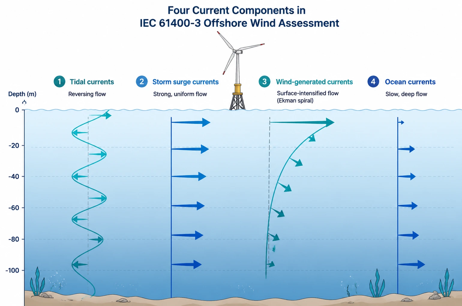
The standard’s most consequential requirement for current measurement: sea currents must be assessed as four independently characterized components:
| Component | Physical Driver | Measurement Implication |
|---|---|---|
| Tidal currents | Astronomical forcing | Predictable, harmonic — requires sufficient duration to resolve spring-neap cycle and principal constituents |
| Storm surge currents | Meteorological forcing during storms | Episodic — requires campaign coverage of storm seasons; the component most vulnerable to seasonal bias |
| Wind-generated currents | Wind stress on sea surface (Ekman processes) | Depth-dependent — requires near-surface current resolution; integrated buoy platforms (Section 3.6) measure wind and current simultaneously |
| Ocean currents | Regional circulation (slope currents, density-driven flow) | Low-frequency — requires long-duration records to separate from tidal signal |
Each component’s velocity and directional characteristics must be assessed separately — a requirement that directly shapes ADCP sampling design: vertical resolution sufficient to distinguish Ekman-influenced surface layers, temporal duration sufficient to separate tidal harmonics from residual flow, and campaign timing covering storm seasons for surge characterization.
2.3 Return Periods: The Extreme Value Requirement
The standard requires extreme sea surface current velocities at 1-year, 50-year, and 500-year return periods, determined from the site-specific metocean database. This single sentence drives the entire statistical structure of a campaign’s data processing (Section 4). Note the standard’s own pragmatism: while site-specific variation of current with depth generally need not be assessed (standard profiles may be assumed), site-specific measurement of current amplitude and direction via ADCP is recommended — and the standard is specific about where: surface currents are especially important for single-point moored floating substructures, and depth variation is especially important for deep-draft floaters.
2.4 Wave Requirements and Joint Probability
Wave assessment requires a joint probability distribution of metocean parameters — wind, waves, and currents together, because the governing design cases involve their simultaneous occurrence. The standard’s resolution requirements are explicit: wind speed bins ≤2 m/s, significant wave height bins ≤0.5 m, wave period bins ≤0.5 s, and wind/wave direction sectors ≤30°. When site-specific measurement data are unavailable, the standard accepts hindcasts or correlations with nearby long-term stations (WAVEWATCH III, long-term buoys) — but the substitution is permitted, not preferred. ADCPs with wave-processing capability contribute directly to this requirement by co-measuring the wave climate (Hm0, Te, directional spectra) alongside currents from the same seabed deployment.
2.5 What the 2025 Floating Standard Changed
IEC 61400-3-2:2025 — the first standalone floating design standard — made three metocean modifications with direct measurement implications:
- Wave directional spreading (new Annexes O and P): highlighted because spreading significantly changes floating turbine loads. Measurement consequence: campaigns must deliver directional wave spectra, not just scalar wave parameters.
- Swell characteristics (new Annex R): long-period swell drives floater resonance responses. Measurement consequence: wave period resolution must separate swell from wind sea — a processing requirement beyond simple Hs/Te reporting.
- Depth-resolved currents for hydrodynamic loading: for floating platforms, hydrodynamic loads depend on water flow kinematics through the full draft depth, and currents affect fluid-inertial loading through convective acceleration. Measurement consequence: depth-profiled currents become a design input, not a check item — favoring full-profile ADCP deployments over single-point meters for floating sites.
3. Deployment Engineering: How the Pros Do It
An ADCP is only as good as the frame that holds it, the anchor that keeps it, and the release system that brings it back. The 2024 field record provides the operational standard.
3.1 Frame Design: The Non-Ferrous Rule
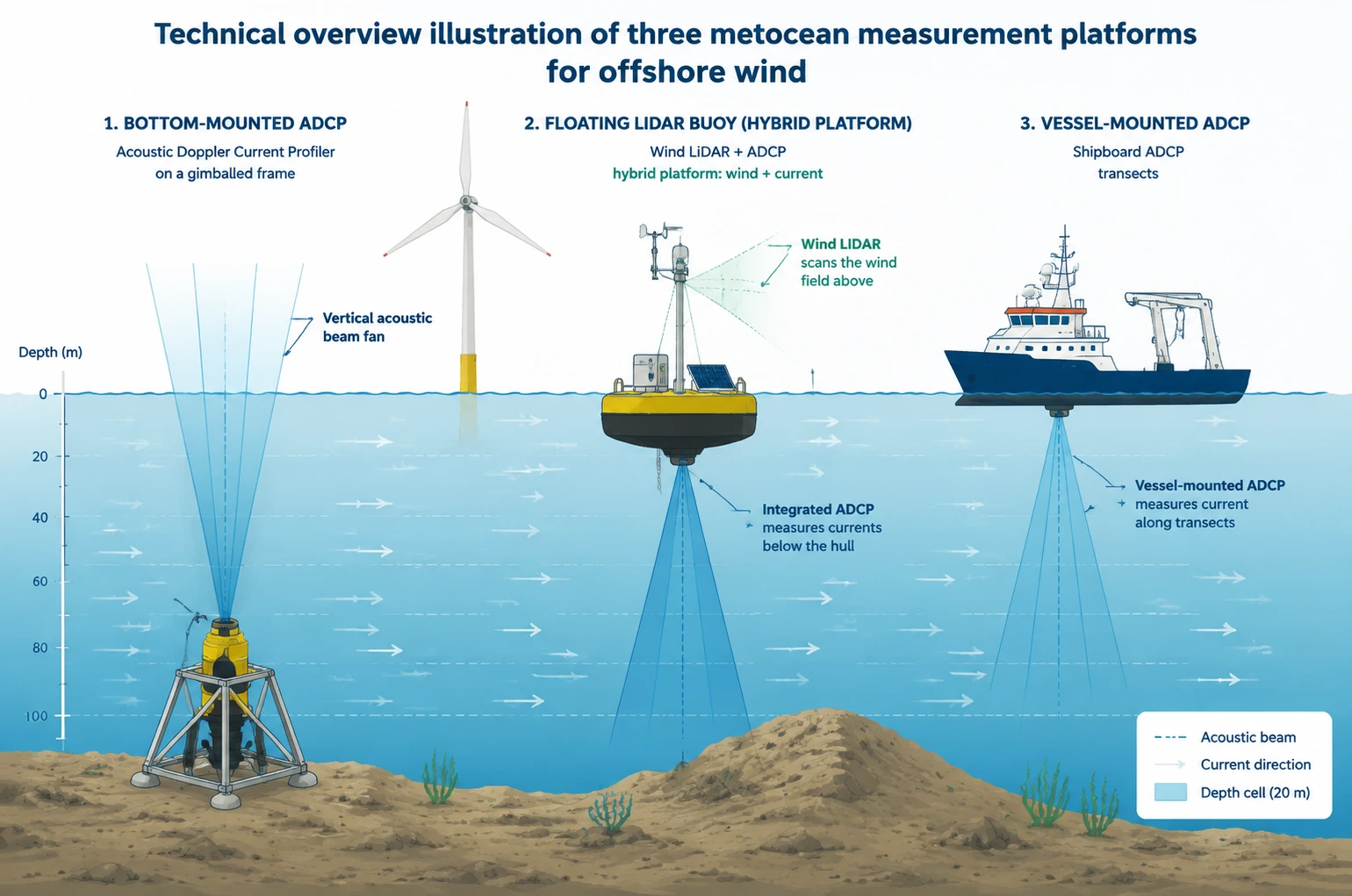
Deployment methodology papers are unanimous on the first design rule: frames must be non-ferrous. The ADCP’s internal fluxgate compass is the reference for current direction — and a ferrous frame distorts it. An incorrect heading corrupts both flow direction and speed measurements, invalidating the entire campaign. The rule extends to connection hardware: non-magnetic stainless steel shackles near the frame, and ground lines that neither float nor billow into the acoustic beams. Second rule: gimballing. The frame gimbals the ADCP so it points vertically through the flow regardless of seabed slope; post-deployment verification (diver or drop camera) confirms levelness. Third rule for long deployments: anti-fouling paint — marine growth on the transducer face degrades signal quality progressively over multi-month campaigns.
3.2 Anchoring: From Self-Weight to Embedded
In calm seabed conditions, ADCP frames hold station by self-weight. In high-flow areas where seabed scour threatens stability, the engineering escalates: gravity-based systems (railway wheels, chain clumps) add mass; direct embedment anchors (screw anchor piles, rock bolts) provide positive holding. The selection is site-driven — a campaign specification should state the expected seabed mobility and specify the anchor class before mobilization, because the anchor choice determines the deployment vessel’s lifting requirements.
3.3 Recovery Systems: The Dual-Acoustic-Release Standard
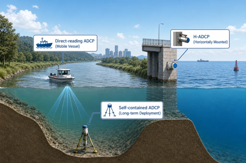
Recovery planning is — in the words of the deployment methodology literature — “among the most important considerations when specifying equipment and marine operations.” The Douarnenez trial (Bay of Douarnenez, France, July 2024) demonstrated the field standard: the ADCP mounted in a gimballed tripod bedframe, deployed via vessel winch line, with dual acoustic releases, rope canisters, and popup buoys for recovery. The dual release provides single-point-of-failure elimination: if one release fails, the second still brings the frame back. Alternative recovery architectures include ground lines and sacrificial bottom moorings with surface marker buoys — each with cost and exposure trade-offs against the trawl and vessel-traffic risks of the specific site.
3.4 Calibration and Metadata: The Pre-Deployment Discipline
Before the frame goes over the side, two tasks are non-negotiable. First, quayside heading calibration: the instrument’s internal magnetic sensor is calibrated on land where the magnetic environment is controlled. Second, site metadata entry: depth, latitude, longitude, and sound velocity are loaded into the instrument so that post-recovery processing can audit every record against known deployment conditions. Campaigns that skip these steps generate data whose audit trail fails under lender’s technical advisor (LTA) review.
3.5 Sampling Strategy: 4 Hz Continuous with Ensemble Averaging
The 2024–2025 operational standard, as demonstrated at Douarnenez: 4 Hz continuous ping logging PD0 data, with edge-computing applications producing 20-minute ensemble averages of mean current for the central 50% of the water column — enabling mid-deployment data review without instrument recovery. For turbulence measurement — required for scour prediction and fatigue analysis — sampling frequencies of 2 Hz or greater (ideally up to 8 Hz) avoid aliasing. Vertical resolution matters equally: meter-scale cells resolve the water-column structure that hydrodynamic models cannot reproduce, and campaigns that coarsen cells to save storage sacrifice exactly the data that model calibration needs.
3.6 Floating LiDAR Buoy Integration: The Hybrid Platform
The Green Rebel configuration (2025) represents the state of the art in integrated metocean measurement: floating LiDAR buoys equipped with ADCPs that sample current profiles to 70 m at up to 8 Hz with ~1 m vertical resolution — measuring wind speed profiles above the surface and current profiles below it simultaneously on one platform. The integration’s scientific value is specific: it captures coupled phenomena such as Ekman processes — wind-driven current response — which matter for understanding how wind stress translates into the current structure that loads foundations and floaters over the project lifecycle. For campaign design, the hybrid platform also consolidates logistics: one deployment, one maintenance schedule, one data pipeline serving both wind and current requirements.
4. From Raw Data to 50-Year Return Currents
The ADCP’s job ends when the frame is recovered. The data’s job is just beginning. The processing chain that converts raw pings into design-grade extreme current values follows a disciplined sequence:
4.1 The Processing Chain
- Coordinate transformation: Beam velocities → Earth coordinates, using the instrument’s heading/pitch/roll — which is why the quayside compass calibration (Section 3.4) is upstream of everything.
- Quality control flagging: Each ensemble is screened against thresholds — correlation counts, percent-good pings, pitch/roll within limits, echo amplitude anomalies — with flagged data excluded from statistics but preserved in the archive.
- Current component separation: Tidal harmonic analysis isolates the tidal constituents; the residual is decomposed into storm surge, wind-generated, and ocean current components per the IEC 61400-3 four-component framework (Section 2.2).
4.2 Extreme Value Analysis
Extreme value analysis is where measured data becomes design criteria. The standard workflow: extract extreme events from the QC’d time series (block maxima by season, or independent peaks above threshold via the peaks-over-threshold method); fit an extreme value distribution (Gumbel for block maxima, Generalized Pareto for peaks-over-threshold); extrapolate to the 1-year, 50-year, and 500-year return levels.
The dominant risk in this chain is seasonal bias: campaigns missing winter storm seasons systematically under-sample the extremes that define the fitted distribution’s tail. Industry analysis of North Sea datasets shows winter-biased data can shift 50-year return current estimates by approximately 35% — an error that propagates directly into foundation design and cable burial specifications. Campaign design that covers at least one complete storm season is therefore not a best-practice nicety; it is the statistical prerequisite for a defensible 50-year value.
4.3 Deliverables That Survive LTA Review
Lender’s technical advisors review metocean deliverables with specific expectations: QC’d data in standardized formats, documented thresholds, and reproducible extreme value analysis. The QC workflow demonstrated at Douarnenez sets the operational bar: dedicated processing software rendering heatmaps of up to 1 terabyte of campaign data, supporting both short surveys and month-long intensive campaigns. For frequency-to-depth matching across the campaign’s depth spectrum, see the ADCP frequency selection guide.
5. Case Studies: What Real Campaigns Discovered
5.1 Anholt OWF, Kattegat, Denmark (August 2024)
A 9-day high-resolution field campaign deployed ADCPs with CT sensors upstream and downstream of an operating monopile. Three findings define its contribution to campaign design practice. First, wind forcing dominated observed variations — confirming the Ekman-driven coupling that integrated wind+current measurement platforms (Section 3.6) are designed to capture. Second, data downstream of the monopile revealed a persistent near-bottom shear layer with enhanced acoustic backscatter — a turbulence and sediment-transport signature that single-point measurements would have missed entirely. Third, and most operationally significant, the study concluded that short-term campaigns are insufficient for capturing full variability of OWF impacts, recommending longer-term monitoring, denser ADCP arrays, and complementary ship-based surveys with vessel-mounted ADCPs and CTD systems. (Source: Tethys/PNNL publication, August 2024.)
5.2 Douarnenez, France (July 2024)
The Sonardyne Origin 600 trial in the Bay of Douarnenez (~33 m depth) demonstrated the complete operational standard for floating-wind site characterization: a >60 m current-profiling ADCP in a gimballed tripod bedframe with dual acoustic releases, quayside heading calibration, site metadata entry, 4 Hz continuous PD0 logging, real-time edge processing with 20-minute ensembles, and post-recovery QC software handling up to 1 terabyte of data. The trial’s operational contribution was proving that real-time mid-deployment data access — previously a direct-reading-only capability — is now available in self-contained configurations through acoustic data download, changing how campaigns monitor their own data health. (Source: Sonardyne trial documentation, July 2024.)
5.3 The Regulatory Pattern: BOEM’s Mooring Expectations
US lease-area practice quantifies the regulatory pattern for campaign scope: BOEM anticipates up to three ADCP moorings per lease area and up to seven along export cable routes, with survey data submitted with the Site Assessment Plan (30 CFR 585.610) and Construction and Operations Plan (30 CFR 585.626). The pattern generalizes internationally: regulators specify minimum spatial coverage; developers exceed it because the marginal cost of an additional mooring is small against the design uncertainty it removes. Survey method statements submitted for marine licences describe the deployment standard: ADCPs in shrouded seabed frames or low-drag submerged buoys, locations selected by depth and seabed character, coordinates submitted for regulatory approval, and total survey durations up to ~12 months including mobilization and demobilization.
6. Equipment Selection Matrix
| Site Type | Water Depth | Recommended Instrument | Key Specifications |
|---|---|---|---|
| Fixed-bottom (nearshore) | 10–70 m | Ocean-ADCP-600-FA4 | 600 kHz, 4-beam Janus, 55–70 m profile, ≥100 days self-contained autonomy, 64 GB storage, ≤10 W |
| Fixed-bottom (transitional) | 70–160 m | Ocean-ADCP-300-FA4 | 300 kHz, 160 m profile, titanium housing to 6000 m |
| Floating wind (deep water) | 160–650 m | Ocean-ADCP-75-PA4 | 75 kHz phased array, 650 m profiling range |
| Buoy/platform point measurement | Any | OCEAN-SPCM | ±0.3% ±3 mm/s, 0.1 mm/s resolution, titanium, 504 Wh battery, PD0 output, 1 Hz |
| Structure-mounted monitoring | Fixed | HADCP-600 | 3-beam, 90 m horizontal range, 2 Hz, RS-232/422 telemetry-ready |
All Oceantek instruments are manufactured under ISO 9001:2015 certified quality management and output industry-standard PD0 format compatible with the processing and QC workflows used in offshore wind metocean campaigns. For the market context driving this measurement demand, see our analysis of offshore wind ADCP demand; for the financial planning perspective, see the companion guide on planning a bankable metocean campaign.
7. Implementation Roadmap: Five Steps to a Compliant Metocean Campaign
| Phase | Duration | Key Activities | Deliverable |
|---|---|---|---|
| 1. Desktop Study | 1–2 months | Hindcast data review; IEC 61400-3 Clause 12 requirement mapping; seasonal bias risk assessment; mooring count and location design | Campaign specification with clause-level requirement traceability |
| 2. Deployment Design | 1 month | Frame fabrication (non-ferrous, gimballed); anchor class selection by seabed mobility; recovery system design (dual acoustic releases); quayside calibration plan | Deployment engineering package + method statement |
| 3. Field Deployment | 3–12 months | Vessel mobilization; frame deployment with metadata entry; mid-campaign data health checks (acoustic download or telemetry); storm season coverage monitoring | Continuous current time series covering at least one storm season |
| 4. Processing and Extreme Value Analysis | 1–2 months | Coordinate transformation; QC flagging; four-component decomposition; extreme value fitting; 1/50/500-year return current computation; seasonal bias verification | QC’d metocean database + extreme value report |
| 5. Delivery and Integration | 2–4 weeks | Standardized format delivery (NetCDF/CSV); LTA review support; integration with design basis and hydrodynamic models | Compliant metocean deliverable package |
8. Frequently Asked Questions
Q: What current measurements does IEC 61400-3 require for offshore wind sites?
IEC 61400-3 (Clauses 6 and 12) requires sea currents assessed as four independently characterized components — tidal, storm surge, wind-generated, and ocean currents — each with its own velocity and directional characteristics. Extreme sea surface current velocities must be determined at 1-year, 50-year, and 500-year return periods from the site-specific metocean database. Site-specific ADCP measurement of current amplitude and direction is recommended, with specific emphasis: surface currents matter most for single-point moored floating substructures; depth variation matters most for deep-draft floaters. The 2025 floating standard (IEC 61400-3-2) adds wave directional spreading (Annex O/P) and swell characteristics (Annex R) to the assessment scope.
Q: How are 50-year return period currents calculated from ADCP data?
The workflow: process raw beam velocities into Earth-coordinate current vectors with full QC flagging; extract extreme events (block maxima or peaks-over-threshold); fit an extreme value distribution (Gumbel or Generalized Pareto); extrapolate to the 50-year return level (annual exceedance probability 0.02). The dominant risk is seasonal bias — campaigns missing winter storm seasons systematically underestimate return-period currents; industry analysis of North Sea data shows winter-biased datasets can shift 50-year estimates by approximately 35%. IEC 61400-3 requires the value from a site-specific database with adequate seasonal and directional coverage.
Q: What frame and anchoring design is used for offshore wind ADCP deployments?
The Douarnenez trial (France, 2024) defines the field standard: ADCP in a gimballed tripod bedframe, deployed via vessel winch, recovered via dual acoustic releases with rope canisters and popup buoys. Design rules from deployment methodology papers: non-ferrous frames (ferrous metal distorts the internal compass and corrupts direction data); gimballing to keep the ADCP vertical; anti-fouling paint for long deployments; and in scour-prone high-flow areas, gravity anchors (railway wheels, chain clumps) or embedded anchors (screw piles, rock bolts) replace self-weight holding. Quayside heading calibration and site metadata entry (depth, coordinates, sound velocity) complete the pre-deployment discipline.
Q: What sampling strategy is used for offshore wind ADCP campaigns?
The 2024–2025 standard: 4 Hz continuous ping logging PD0 data, with edge processing producing 20-minute ensemble averages of mean current for the central 50% of the water column — enabling mid-deployment review without recovery. Turbulence measurement requires 2 Hz or greater (ideally up to 8 Hz) to avoid aliasing. Meter-scale vertical cells resolve water-column structure that models cannot reproduce. Floating LiDAR buoy integrations (Green Rebel, 2025) sample profiles to 70 m at 8 Hz with ~1 m resolution, measuring wind above and currents below the surface simultaneously to capture Ekman coupling.
Q: What is different about metocean measurement for floating offshore wind?
IEC 61400-3-2:2025 (the first standalone floating standard) imposes three distinct demands. Depth-resolved currents: floating platforms have deep drafts, and current depth variation affects hydrodynamic loading through convective acceleration — full-profile ADCPs become design inputs, not check items. Wave directional spreading (new Annexes O and P): spreading significantly changes floating turbine loads, requiring directional wave spectra. Swell characterization (new Annex R): long-period swell drives floater resonance, requiring wave period resolution separating swell from wind sea. With floating capacity at 278 MW operational and a 244 GW pipeline, these requirements define the industry’s fastest-emerging measurement standard.
Q: What did the Anholt and Douarnenez campaigns teach about campaign design?
The Anholt study (Denmark, August 2024) deployed ADCPs with CT sensors around an operating monopile for 9 days: wind forcing dominated variability; a near-bottom shear layer with enhanced backscatter appeared downstream of the monopile; and the study concluded short campaigns are insufficient — recommending longer monitoring, denser ADCP arrays, and vessel-mounted surveys. The Douarnenez trial (France, July 2024) proved the operational standard: gimballed frame with dual acoustic releases, 4 Hz continuous PD0 logging, real-time 20-minute ensembles, and QC software handling 1 terabyte of data. Together: temporal duration and operational reliability are the two axes of campaign quality.
Q: What equipment does Oceantek offer for offshore wind metocean campaigns?
Oceantek covers the full depth spectrum: Ocean-ADCP-600-FA4 (600 kHz, 55–70 m, ≥100 days autonomy) for nearshore fixed-bottom sites; Ocean-ADCP-300-FA4 (160 m, titanium) for transitional depths; Ocean-ADCP-75-PA4 (75 kHz phased array, 650 m) for floating wind and deep water; OCEAN-SPCM (±0.3% ±3 mm/s, 504 Wh battery) for buoy point measurement; and HADCP-600 (90 m horizontal) for structure-mounted monitoring. All output PD0 format and are manufactured under ISO 9001:2015 certified quality management.
9. Conclusion
The offshore wind industry’s 441 GW ambition rests on a measurement foundation that is young but maturing fast. The standards are now specific — four current components, three return periods, joint probability distributions, and a 2025 floating edition that sharpens every requirement. The deployment engineering is now proven — non-ferrous gimballed frames, dual acoustic releases, 4 Hz continuous logging with real-time ensembles. The statistical discipline is now understood — extreme value analysis whose dominant risk is the seasonal gap that short campaigns leave behind.
For developers, consultancies, and marine contractors, the technical substance of an ADCP metocean campaign is this: measure the right components at the right resolution for the right duration, deploy it so it comes back, and process it so it survives review. Oceantek’s instruments — from the Ocean-ADCP-600-FA4 for nearshore campaigns to the Ocean-ADCP-75-PA4 for floating-wind depths — provide that measurement layer, manufactured under ISO 9001:2015 certified quality management and compatible with the industry’s standard PD0 workflows.
Research Methodology: This article draws on 12+ primary sources including: IEC 61400-3:2009, IEC 61400-3-1:2019, and IEC 61400-3-2:2025 (design requirements for offshore wind turbines, with Clause 6 and Clause 12 metocean requirements); GWEC Global Wind Report 2026 (83 GW cumulative 2024, 441 GW by 2034); World Forum Offshore Wind statistics (78.5 GW operational, floating 278 MW/244 GW pipeline); Tethys/PNNL Anholt OWF field campaign study (August 2024); Sonardyne Origin 600 Douarnenez trial documentation (July 2024); Green Rebel floating LiDAR buoy integration (ECO Magazine, Spring 2025); Hydro International coverage of Partrac/Nortek floating wind metocean services; BOEM site characterization guidance (30 CFR 585.610/626, mooring expectations); EWTEC ADCP deployment methodology paper (frame design, anchoring, compass calibration); and Oceantek product specifications for Ocean-ADCP-600-FA4, Ocean-ADCP-300-FA4, Ocean-ADCP-75-PA4, OCEAN-SPCM, and HADCP-600.
Disclosure: Oceantek designs and manufactures acoustic Doppler current profilers and Doppler velocity logs at its ISO 9001:2015 certified facility in Hangzhou, China. The product recommendations in this article reflect Oceantek’s instrument portfolio, selected to illustrate the deployment configurations and selection principles applicable to offshore wind metocean campaigns. References to Nortek, Sonardyne, Teledyne RDI, and other manufacturers reflect actual instruments used in the cited studies and trials.
Last updated: August 21, 2026.