Executive summary
A pulse-coherent ADCP is not a higher-accuracy version of a conventional current profiler. It is a different measurement approach that trades profiling range and measurable velocity range for very fine spatial and temporal resolution. It resolves velocity structure over centimetres by comparing the phase of echoes from a pair of short pulses, and it fails in a characteristic way when the flow is too fast or the profile too long for its pulse separation. This article explains the mechanism, the range-velocity trade-off that governs every configuration, how it compares with narrowband and broadband processing, and where the method is worth its constraints.
Contents
- What is a pulse-coherent ADCP?
- How does pulse-coherent ADCP work?
- Why does it provide higher resolution?
- The critical trade-off: range versus velocity
- Pulse-coherent vs narrowband vs broadband
- When should you use a pulse-coherent ADCP?
- When should you not use one?
- How to choose pulse-coherent settings
- Practical limitations and common errors
- Pulse-coherent ADCP in real research
- Quick comparison
- Frequently asked questions
- Conclusion
1. What is a pulse-coherent ADCP?
1.1 Definition of pulse-coherent Doppler processing
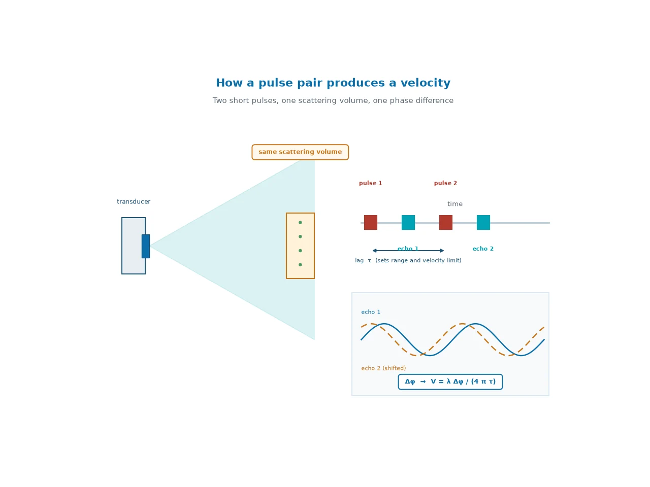
A pulse-coherent ADCP — more precisely, a pulse-to-pulse coherent profiler — measures velocity from the phase difference between two echoes returned by two successive short acoustic pulses. The first pulse travels into the water, scatters from particles in a small volume, and returns. After a fixed delay the instrument transmits a second pulse and receives the echo from the same volume. The phase of the two echoes differs by an amount proportional to how far the scatterers moved along the beam between the pulses.
ISO 24578 groups ADCP signal processing into three families: pulse-incoherent, pulse-to-pulse coherent and broadband. The same standard notes that coherent processing can deliver very low short-term velocity uncertainty while being limited in measurement distance and maximum velocity. Those two sentences summarise the whole method: excellent precision, restricted operating envelope. The measurement concept itself builds on the Doppler principle described in our guide to how an ADCP works.
1.2 What "coherent" means here
Coherence refers to the assumption that the scattering field has not rearranged significantly between the two pulses. If the particles in the sampled volume stay correlated, the phase difference is a clean measure of displacement. If the water mixes the scatterers too quickly — strong turbulence, breaking waves, dense bubble clouds — correlation is lost and the velocity estimate degrades. This is why pulse-coherent systems are used at short range in moderate conditions rather than at long range in energetic ones.
2. How does pulse-coherent ADCP work?
2.1 Short-pulse transmission
Cell size is set by pulse length, approximately half the sound speed multiplied by the pulse duration. A 1 cm cell therefore requires a pulse of about 13 microseconds in seawater. That is very short compared with the pulses used by narrowband profilers, and it is the origin of the technique's spatial resolution. The pulse itself is generated by the transducer, which converts electrical energy into sound through piezoelectric ceramic elements.
Short pulses carry less energy, so the echo is weaker and the signal-to-noise ratio is lower for a single ping. The instrument compensates by averaging, which is one reason the sampling strategy matters as much as the pulse length.
2.2 Transmitting the pulse pair
The instrument transmits pulse 1, waits for its echo, then transmits pulse 2 after a defined lag. Both pulses must illuminate the same volume for the phase comparison to be valid. The lag — the time between the two transmissions — is the single most important setting in a pulse-coherent profile, because it sets both the maximum range and the unambiguous velocity.
2.3 Measuring the phase change
The relationship between phase difference and radial velocity is direct:
Vr = λ · Δφ / (4π · τ)
where Vr is the radial velocity along the beam, λ is the acoustic wavelength, Δφ is the phase difference between the two echoes and τ is the pulse separation. Because the phase is measured over a full acoustic cycle, the technique is very sensitive: small displacements produce measurable phase shifts. The same periodicity, however, creates the ambiguity discussed in section 4.
2.4 From radial velocity to three-dimensional velocity
Each beam measures velocity along its own axis. Combining the radial velocities from a multi-beam array resolves the horizontal and vertical components, provided the instrument knows its attitude and heading. Beam geometry therefore determines what the instrument can resolve and how much redundancy it has when one beam is contaminated. In a phased-array design the beams are formed electronically, which keeps the transducer face flat; in a piston design each beam comes from a separate tilted element. The options are compared in our article on 4-beam, 5-beam and 9-beam configurations.
3. Why does pulse-coherent ADCP provide higher resolution?
3.1 Shorter pulses and smaller measurement cells
Range resolution follows pulse length, so reducing the pulse from metres to centimetres reduces the cell by the same factor. Published experiments using pulse-coherent profilers have reported vertical cells of the order of 0.01 to 0.02 m, and a study of near-bed suspended sediment flux used cells of roughly 0.7 cm. Those figures come from specific instruments and configurations rather than from the method in general, but they show what the technique makes possible: a profile of the lowest metre of the water column with the same number of cells that a conventional profiler would use to cover tens of metres.
3.2 Lower short-term measurement uncertainty
Resolution is only useful if the velocity estimate is precise enough to exploit it. Phase-based measurement gives pulse-coherent instruments low short-term uncertainty, which is why they are used for turbulence work where the signal of interest is a fluctuation rather than a mean. A one-centimetre cell is pointless if the velocity noise in that cell is larger than the fluctuation being studied.
3.3 Higher temporal resolution
Because each measurement uses a short pulse pair rather than a long pulse, more estimates can be produced per unit time, which matters when the process being observed evolves on a wave period or a turbulent timescale. There is a trade-off here as well: a higher output rate leaves fewer pings to average, so the statistical uncertainty of each estimate can rise. Section 8.4 covers how to balance the two.
4. The critical trade-off: range versus velocity
4.1 Why profiling range is limited
The second pulse cannot be transmitted until the echo from the first has returned from the far end of the profile. Otherwise the instrument cannot tell which pulse produced a given echo. That constraint sets the maximum range:
Rmax ≈ c · τ / 2
With a sound speed of about 1,500 m/s, a 2 ms lag corresponds to roughly 1.5 m of range, a 10 ms lag to about 7.5 m, and a 50 ms lag to about 37 m. Pulse-coherent profilers are therefore short-range instruments by construction: they are designed to look at metres, not hundreds of metres.
4.2 What is velocity ambiguity?
Phase is periodic. If the scatterers move far enough between the two pulses, the measured phase difference can no longer be distinguished from the difference produced by a slower movement plus one full cycle. The velocity that corresponds to a half-cycle of phase is the unambiguous limit:
Vamb = ± λ / (4 · τ)
At 1 MHz, where the wavelength is about 1.5 mm, a 10 ms lag gives an unambiguous velocity of about 3.8 cm/s. A flow of 0.3 m/s would not be measured as 0.3 m/s; it would fold back into the ambiguous range. This is the failure mode that ISO 24578 warns about: if the coherent processing range or the maximum velocity limit is exceeded, the data can become meaningless rather than merely noisy.
4.3 The range-velocity trade-off
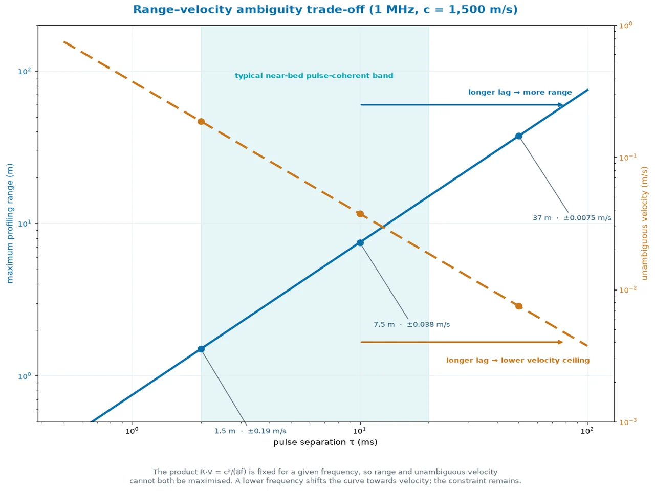
Multiplying the two expressions shows why the trade-off cannot be avoided:
Rmax · Vamb ≈ c² / (8 f)
For a given acoustic frequency, the product of range and unambiguous velocity is a constant. A 1 MHz instrument can offer about 1.5 m of range with ±0.19 m/s of unambiguous velocity, or 7.5 m with ±0.038 m/s — but never both together, because the operating point always sits somewhere on the same curve. Lowering the frequency enlarges the wavelength and moves the whole curve in favour of velocity; the constraint itself remains.
4.4 How ambiguity can be managed
- Multiple lags. Repeating the measurement with different pulse separations produces complementary ambiguity patterns that can be resolved in processing.
- Frequency choice. A lower frequency increases the unambiguous velocity for the same lag, at the cost of a larger transducer and coarser cells.
- Accepting a shorter range. In near-bed work the profile of interest is often only one to three metres, which relaxes the constraint considerably.
- Using a different processing mode. Where the objective is a long profile or a wide velocity range, broadband or pulse-incoherent processing is the appropriate choice rather than an adjustment to the coherent configuration.
- Cross-checking with independent data. Temperature, salinity or a second instrument can reveal that a velocity record folded into the ambiguous range.
5. Pulse-coherent vs narrowband vs broadband ADCP
5.1 Pulse-incoherent / narrowband
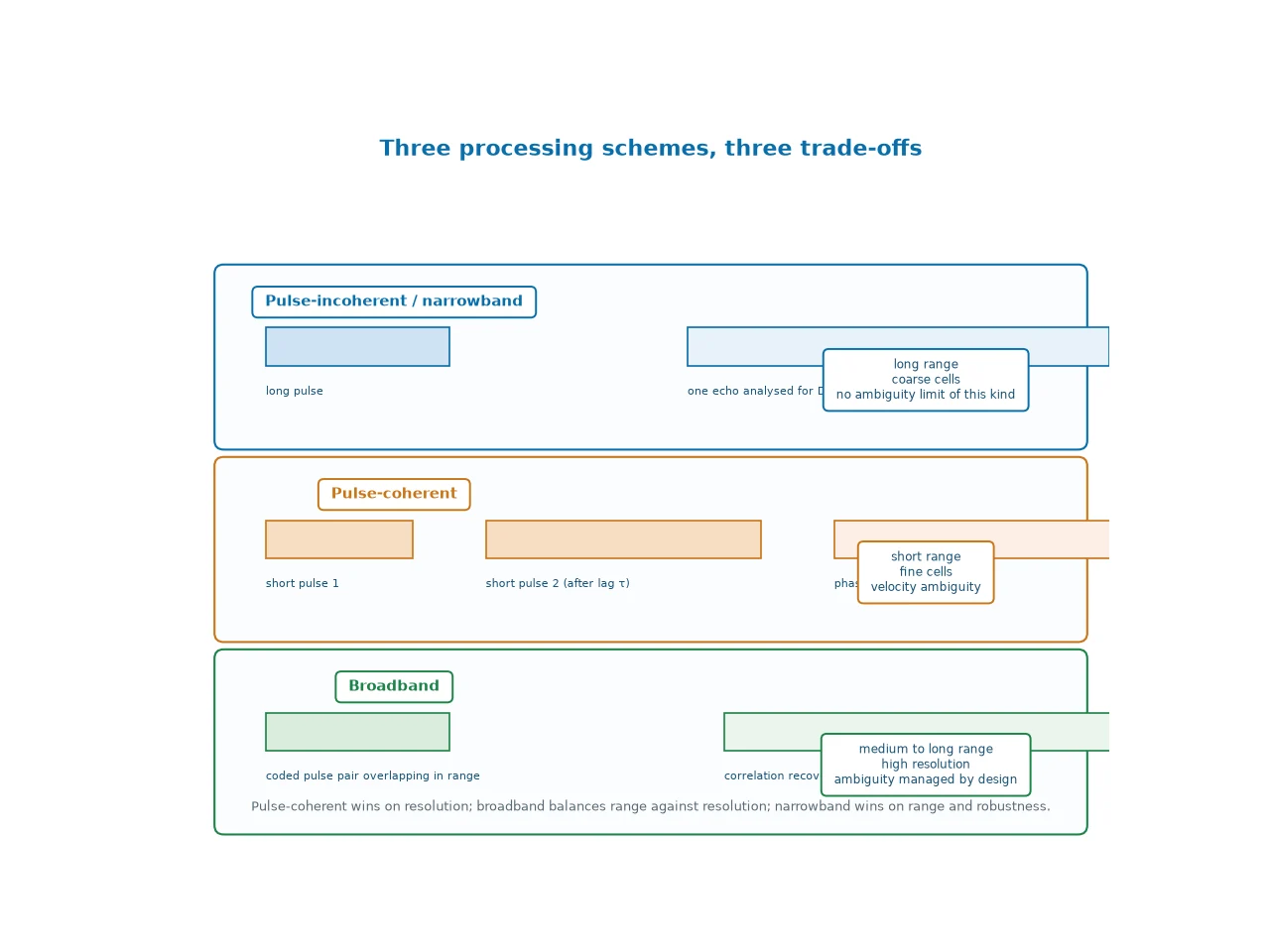
A narrowband profiler transmits a relatively long pulse and estimates the Doppler shift from the frequency content of the echo. The method is robust and reaches long ranges, but cell size is set by the long pulse, so vertical resolution is coarse. It remains a reasonable choice for large-scale flow where fine structure is not the objective.
5.2 Pulse-coherent
As described above: two short pulses, a phase comparison, excellent short-term precision and centimetre-scale cells, limited by range and by velocity ambiguity.
5.3 Broadband
Broadband processing also uses pulse pairs and phase information, but the pulses are coded and may be present in the water at the same time; range and velocity are recovered by correlation. ISO 24578 describes this as the difference that distinguishes broadband from pulse-coherent processing. The practical consequence is a longer unambiguous profile and a wider usable velocity range, with resolution that is good but not as fine as a dedicated coherent configuration.
5.4 Which processing approach fits which measurement?
| Processing | Basic approach | Main strength | Main limitation |
|---|---|---|---|
| Pulse-incoherent / narrowband | Doppler frequency from a long single pulse | Long range, robust in difficult conditions | Coarse vertical resolution |
| Pulse-coherent | Phase difference between successive short pulses | Very fine resolution, low short-term uncertainty | Short range, low unambiguous velocity |
| Broadband | Coded pulse pair with correlation processing | Balances range and resolution over a wide velocity range | Not as fine-scale as a coherent configuration |
6. When should you use a pulse-coherent ADCP?
6.1 Near-bed velocity measurement
The lowest metre of the water column is where bed friction, sediment transport and structure interaction are decided. Conventional profilers resolve it poorly because their cells are larger than the layer itself. A pulse-coherent profile with centimetre cells describes the velocity gradient directly.
6.2 Sediment transport and suspended sediment
Suspended sediment flux is the product of concentration and velocity, both of which vary sharply near the bed. Fine cells make it possible to compute flux profiles rather than bulk estimates. The measurement approach is described in our article on ADCP sediment monitoring.
6.3 Boundary-layer research
Boundary layer studies need velocity at a resolution comparable to the scales of the processes being investigated — shear production, bed roughness, wave-current interaction. Pulse-coherent profilers have been used in this role for decades, including in coastal and estuarine field campaigns.
6.4 Turbulence measurements
Turbulence work needs both fine spatial resolution and low noise, which is precisely the combination that phase-based processing provides. The limitation is that the method assumes the flow field is reasonably uniform across the beam spread; strong lateral gradients violate that assumption.
6.5 Fine-scale ocean current structure
Autonomous and moored pulse-coherent instruments have been used to observe centimetre-scale velocity structure in the open ocean, including internal wave and fine-shear studies, where ambiguity is handled explicitly in processing.
7. When should you not use a pulse-coherent ADCP?
7.1 Long-range profiling
If the profile needs to reach tens or hundreds of metres, the pulse separation required would reduce the unambiguous velocity to a value far below the flow. Long profiles belong to broadband or pulse-incoherent instruments.
7.2 High-velocity flows
River discharge measurement, tidal straits and industrial channels routinely exceed the unambiguous velocity of a short-lag coherent configuration. A record that aliases is not a degraded measurement; it is a wrong one. For river work, see our guide to river discharge measurement.
7.3 Deep-water full-depth measurements
Full-depth ocean profiles are a broadband or narrowband application. Instruments used for this work are described in our article on deep-sea current measurement.
7.4 Conditions beyond the ambiguity limit
ISO 24578 is explicit that when the coherent processing range or maximum velocity limit is exceeded, the measurement data may lose validity. A configuration should be checked against the site's expected maximum velocity and required range before deployment, not after the data are processed.
8. How to choose pulse-coherent ADCP settings
8.1 Acoustic frequency
Frequency sets wavelength, which sets both the unambiguous velocity for a given lag and the acoustic attenuation. Higher frequencies give finer resolution and better small-particle scattering but shorter range and a lower velocity ceiling. Frequency selection is treated in more detail in our ADCP frequency selection guide.
8.2 Pulse separation / lag time
The lag is the operating point on the range-velocity curve. Choose it from the two requirements that matter — the depth of the layer to be resolved and the highest velocity expected — and verify that both sit inside the envelope with margin.
8.3 Cell size
Cell size follows pulse length. Very thin cells increase resolution but reduce the number of scatterers per cell and therefore the signal-to-noise ratio, which has to be recovered by averaging. The configuration guides cover the cell count and range relationship for profiling instruments in general: ADCP configuration.
8.4 Sampling rate and averaging
Higher output rates are not automatically better. Each pulse pair occupies time, so a faster sampling scheme leaves fewer independent estimates to average, and the statistical uncertainty of each velocity estimate can increase. In wave-dominated or turbulent conditions the sampling scheme should be matched to the timescale of the process, not maximised.
8.5 Signal-to-noise ratio and acoustic scattering
An ADCP measures particles moving with the water, not the water itself. Suspended sediment, bubbles, plankton and other scatterers determine how much signal returns. In clear water the range may be shorter than the geometric limit; in sediment-laden water the signal is strong but the scatterers may decorrelate faster. Both effects belong in the deployment plan.
9. Practical limitations and common measurement errors
9.1 Velocity aliasing
Flow faster than the unambiguous velocity appears as a plausible but incorrect value. Checking the record against tide, river stage or an independent current measurement is the standard defence.
9.2 Loss of correlation
If the scattering field changes too much between pulses, the phase comparison loses meaning. The symptom is elevated noise or dropouts rather than a systematic offset.
9.3 Near-field and acoustic effects
Close to the transducer the beam has not formed fully, and ringing or near-field effects contaminate the first cells. Cell one is not always a usable cell.
9.4 Low backscatter
Clear, particle-poor water weakens the echo. Deployment height and averaging have to compensate, or the profile will be shorter than the specification suggests.
9.5 Excessive flow velocity
Related to aliasing but distinct in practice: a site that occasionally exceeds the ambiguity limit produces intermittent bad data rather than a consistently wrong record, which is easy to miss if only mean values are reviewed.
9.6 Incorrect pulse separation
A lag chosen for range rather than for the expected velocity is one of the most common configuration errors. Both constraints must be evaluated together.
9.7 Side-lobe interference and boundary effects
Near a boundary, energy returned through the side lobes can reach the transducer before the main lobe has travelled to the bed, so there is a minimum standoff distance below which the measurement is unreliable. High resolution near the bed does not mean unlimited access to the bed itself. Boundary interference is also relevant to structures and outfalls, as discussed in our article on outfall monitoring.
10. Pulse-coherent ADCP in real research
Three published applications show where the method has been used rather than merely described.
10.1 Near-bed sediment transport
A coastal field study used a coherent Doppler profiler to measure near-bed suspended sediment flux at a vertical resolution of roughly 0.7 cm, resolving the interaction between bed forms and flux. The study is a useful reference for how fine cells change what can be computed rather than merely observed.
10.2 Bottom boundary layer turbulence
Coherent profilers have been applied to turbulence measurement in the bottom boundary layer, using high-resolution velocity series to estimate turbulence characteristics. The requirement is the combination of fine cells and low noise; either alone is insufficient.
10.3 Fine-scale ocean velocity structure
Autonomous pulse-coherent instruments have been used to observe centimetre-scale velocity structure in the open ocean, with phase ambiguity handled explicitly in processing. This is the clearest demonstration that the method's range limitation is a design constraint rather than a barrier to scientific use.
11. Quick comparison
| Feature | Pulse-incoherent | Pulse-coherent | Broadband |
|---|---|---|---|
| Spatial resolution | Lower | Very high | High |
| Short-term precision | Lower | Very high | High |
| Profiling range | Long | Short | Medium to long |
| Velocity ambiguity | Different limitation | Important constraint | Managed by design |
| Near-bed studies | Limited | Excellent | Good |
| Turbulence work | Limited | Excellent | Good |
| Long-range profiling | Excellent | Limited | Excellent |
| Sediment boundary layer | Limited | Excellent | Good |
The table is not a ranking. Each processing scheme is matched to a measurement objective, and programmes that need both fine-scale and long-range data often deploy instruments in different modes rather than asking one configuration to do everything.
12. Frequently asked questions
What is a pulse-coherent ADCP?
It is a current profiler that measures velocity from the phase difference between echoes returned by two successive short pulses from the same scattering volume. Pulse-to-pulse coherent processing is one of the three signal-processing families described in ISO 24578, alongside pulse-incoherent and broadband processing.
How does a pulse-coherent ADCP measure velocity?
It transmits a short pulse, receives the echo, waits a set lag, transmits a second short pulse, and compares the phase of the two echoes. The phase difference is proportional to radial velocity along the beam. Multiple beams resolve the three-dimensional velocity.
Why does pulse coherence improve spatial resolution?
Cell size is set by pulse length, roughly half the sound speed multiplied by the pulse duration, so a short pulse produces a thin cell. Published experiments using pulse-coherent profilers have reported cells of 0.01 to 0.02 m, and one near-bed sediment study used roughly 0.7 cm cells.
What is velocity ambiguity in a pulse-coherent ADCP?
Phase can only be measured within a cycle, so the velocity producing a half-cycle phase shift sets an upper limit: the unambiguous velocity is the wavelength divided by four times the lag. Flows faster than that limit appear aliased to a lower velocity.
What is the difference between pulse-coherent and broadband ADCP?
Both use pulse pairs and phase information. A pulse-coherent system waits for the first echo before sending the second pulse, which limits its range. A broadband system transmits coded pulses that can be in the water simultaneously and recovers range and velocity by correlation, trading resolution for a longer profile.
How far can a pulse-coherent ADCP measure?
Maximum range is approximately half the sound speed multiplied by the pulse lag: about 1.5 m at a 2 ms lag, 7.5 m at 10 ms, and 37 m at 50 ms. Range and unambiguous velocity cannot both be maximised because their product is fixed by frequency.
Is pulse-coherent ADCP suitable for river discharge measurement?
Usually not as the primary mode. Discharge measurement needs a full-depth profile and often involves flow speeds above the unambiguous velocity of a short-lag coherent configuration. Broadband or pulse-incoherent processing is normally used for discharge work.
When should I use pulse-coherent instead of broadband?
Use pulse-coherent when the objective is a thin layer: near-bed velocity, suspended sediment flux, boundary layer turbulence or centimetre-scale shear. Use broadband when the objective is a longer profile, a wider velocity range, or routine discharge measurement.
13. Conclusion
Pulse-coherent processing is not simply a higher-accuracy version of conventional ADCP technology. It is a specialised measurement approach designed to resolve fine-scale velocity structures when a short profiling range and a limited unambiguous velocity can be managed. Three questions decide whether it is the right tool: how fine the velocity structure has to be resolved, how far the profile has to reach, and how fast the water moves. Where the answers point to centimetres and metres rather than tens of metres, pulse-coherent mode is the only way to obtain that detail.
Where the objective is a longer profile or a wider velocity range, the same instruments offer broadband or pulse-incoherent modes, and the configuration choices are set out in our guidance on key ADCP selection parameters. Where the measurement is going to be reported formally, the uncertainty framework in ISO 25377 applies to the derived quantities.
Published by Oceantek engineering team.Lasted update:September 24,2026.