Executive Summary
Every coastal city operates infrastructure that is simultaneously essential and invisible: the ocean outfall. Designed for 25–50 year service lives, these submarine pipelines discharge treated effluent through multiport diffusers and rely on ocean currents to dilute it to regulatory standards. Whether that dilution actually happens — at the required ratio, within the permitted mixing zone — is a measurement question. And the instrument at the center of that measurement is the ADCP.
This guide covers the science of effluent dilution, the ADCP deployment methodologies proven across six international monitoring programs (Boston, Sydney, Rio de Janeiro, Honolulu, San Diego, Hong Kong), the regulatory frameworks governing mixing zones in the US, Australia, and Europe, and the fastest-growing application of all: desalination brine discharge monitoring.
Table of Contents
1. Introduction: The Invisible Infrastructure
Ocean outfalls are the least-visible component of urban water infrastructure — kilometers of submarine pipeline terminating in multiport diffusers on the seabed, discharging treated effluent into the coastal ocean. They are also among the longest-lived: designed for 25–50 year service lives, often operating at low initial flows and reaching design capacity only decades after construction.
That longevity creates a monitoring problem with high stakes. An outfall approved on the basis of modeled dilution may operate for years under conditions that differ from its design assumptions — currents shift, stratification regimes change with climate, diffuser ports clog with marine growth, and flow rates climb toward design capacity. Regulatory compliance, public health, and benthic ecosystem protection all depend on verifying that actual dilution matches predicted dilution — and the ADCP is the instrument that makes that verification possible.
Three measurement questions define outfall monitoring:
- Where does the plume go? — answered by long-term ADCP current characterization: the ambient velocity field that advects and spreads the effluent.
- How diluted is it? — answered by dye tracer studies integrated with real-time ADCP current data: the measured dilution factor compared against regulatory mixing-zone requirements.
- What depth does it occupy? — answered by combining ADCP current profiles with CTD density structure: whether the plume surfaces, traps at the thermocline, or hugs the seabed.
2. The Science of Effluent Dilution
2.1 Near-Field vs. Far-Field Dilution
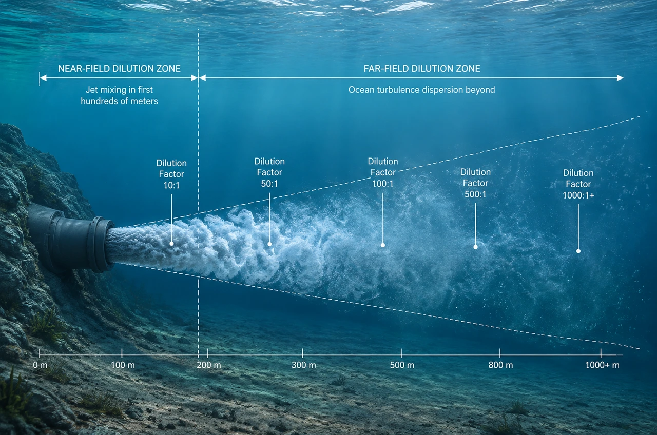
Effluent dilution proceeds in two distinct regimes, and monitoring programs must address both:
| Regime | Spatial Extent | Driving Mechanism | Typical Dilution Achieved | Primary Measurement Method |
|---|---|---|---|---|
| Near-field | First tens to hundreds of meters from diffuser | Discharge-generated turbulence — jet entrainment and mixing at the diffuser ports | Hundreds (Sydney deepwater outfalls: 200:1–300:1 initial dilution) | Dye tracer + CTD profiling close to diffuser |
| Far-field | Beyond, to kilometers | Ocean current advection + oceanic turbulence diffusion | Typically <10× additional | Long-term ADCP current time series + trajectory modeling (RSB/CORMIX/JETLAG) |
The Hong Kong NWNT outfall study validated this two-stage structure with radioactive tracers: dilution was achieved mainly in the near-field (hundreds), with far-field processes adding roughly another order of magnitude. The operational consequence for monitoring design: near-field measurement is a survey problem (tracer releases during targeted cruises), while far-field prediction is a current measurement problem (continuous ADCP time series feeding trajectory models).
2.2 Measuring the Dilution Factor: Dye Tracer Methodology
The dilution factor — the regulatory metric for outfall performance — is measured with tracer techniques:
- Tracer injection: Rhodamine WT (the industry standard; Uranine and Amidorhodamine G are alternatives) is injected continuously into the outfall pipeline at known concentration and flow rate for 6–8 hours. For far-field work, radioisotopes (gold-198, tritium, technetium) offer a detection volume six orders of magnitude larger than fluorometers.
- Plume mapping: Fluorometers mounted on CTD profilers or tow-yo systems map the dye field along transects. At Sydney’s deepwater outfalls, CTD was found most effective for near-field characterization; technetium radioisotopes covered the near-to-far-field transition.
- Dilution calculation: Dilution = effluent tracer concentration ÷ measured receiving-water concentration at each sample point. Sydney measured initial dilutions of 200:1 to 300:1; the Ipanema (Rio de Janeiro) program quantified affected areas for dilution factor bands (30–50, 51–100, 101–200).
- ADCP integration: The concurrent ADCP current data provides the physical interpretation — at Ipanema, dye tracer plumes showed perfect agreement with ADCP-measured current direction, confirming that the ambient current field governs plume advection and validating the combined measurement architecture.
2.3 Stratification: The Invisible Control on Plume Depth
Whether a diluted plume surfaces — where beach water quality and public health are directly affected — or remains trapped below the thermocline is governed by density stratification. The monitoring requirement is therefore to characterize stratification alongside currents:
- At the Ipanema outfall, the water column was nearly homogeneous over 80% of the year, supporting the use of simpler 2D water quality models; during the ~20% stratified periods, plume trapping depth was inferred from temperature profiles.
- At Sydney’s deepwater outfalls, plumes were observed trapped below 30–60 m depth depending on thermocline conditions, with currents varying from 0.4 m/s at 15 m depth to 0.15 m/s at 50 m.
- At Mamala Bay (Hawaii), a downward-looking ADCP moored with a 14-thermistor string at 10-foot intervals measured velocity and temperature at one-minute resolution, capturing the internal-wave-driven variability that modulates mixing. Professor Philip Roberts’ related studies used 300 kHz ADCPs recording at half-hour intervals; the RSB model then predicted seasonal surfacing — 11% of summer and 28% of winter.
2.4 Dense Plumes: The Special Physics of Brine
Industrial discharges that are denser than seawater — most notably desalination brine — invert the classic plume picture. The negatively buoyant jet discharged at the standard 60° inclination rises on initial momentum, then collapses back to the seabed under negative buoyancy, spreading as a bottom-hugging density current. Dilution continues as the density current flows down-slope, but the environmental footprint concentrates on benthic ecosystems: Mediterranean studies measured brine-amended sediments with ~6-fold higher dissolved organic phosphorus influx, 15% increased oxygen consumption, and 1.5–6.5-fold increased microbial activity. Dense-plume monitoring therefore demands seabed-focused measurement strategies — a requirement explored in Section 5.
3. ADCP Monitoring Methods
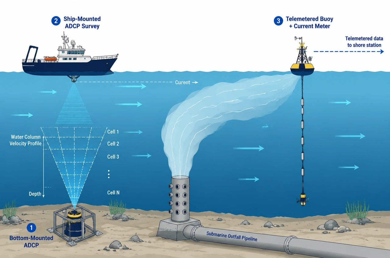
Six internationally documented monitoring programs establish the ADCP deployment patterns for outfall applications. Three configurations dominate:
3.1 Bottom-Mounted Long-Term Current Characterization
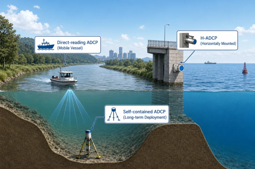
The foundational dataset for any outfall program is a multi-month current time series at the diffuser site. The Ipanema outfall (Rio de Janeiro) provides the reference deployment: an ADCP programmed to measure 9 depth layers, paired with an 11-sensor thermistor string, deployed near the diffusers for one full year, sampling every 30 minutes. The results defined the site’s hydrodynamic regime precisely — currents below 20 cm/s for 78–80% of the time, predominant directions parallel to the coast (azimuths 60° and 240°), and a homogeneous water column over 80% of the year. Spectral analysis further separated the forcing: surface circulation driven by meteorological events (cold fronts), bottom circulation tide-dominated. This depth-resolved, season-resolved current characterization is exactly what the Ocean-ADCP-600-FA4 (≥100 days self-contained autonomy, 64 GB storage) delivers for coastal outfall depths, with the Ocean-ADCP-300-FA4 extending coverage to 160 m for deepwater outfalls.
3.2 Ship-Mounted Real-Time Plume Tracking Surveys
During dye tracer experiments, a ship-mounted ADCP provides the real-time current context that converts a dye map into a physically interpretable dilution measurement. The MWRA Boston outfall program used a ship-mounted 600 kHz ADCP collecting current profiles at 0.5–1.0 m vertical increments between 2.5 and 26 m depth, operated continuously during offshore survey days while dye was emerging from the diffusers. The USGS supplemented this with a bottom-mounted ADCP moored approximately 1,000 m south of the diffuser, providing the long-term reference current series. The combination — survey-time real-time currents plus deployment-period mean currents — is the standard architecture for near-field interpretation.
3.3 Telemetered ADCP Driving Adaptive Sampling
The most operationally advanced pattern comes from San Diego’s Point Loma outfall: telemetered ADCP and temperature data from a permanent mooring at the terminal diffuser wye were used to compute 72-hour water-column trajectory estimates, updated hourly, which guided autonomous underwater vehicle (AUV) mission planning for plume sampling. The AUV carried its own 1200 kHz ADCP for navigation (altitude and speed over seafloor) alongside CTD and fluorometer payloads, tracking dilution to over 9 km from the diffusers. This adaptive monitoring architecture — long-term mooring forecasts the plume, mobile platforms verify it — represents the state of the art and aligns with NPDES recommendations to integrate telemetered data into adaptive sampling grid design. The OCEAN-SPCM (titanium housing, 504 Wh battery, months of unattended operation) provides the buoy-mounted current measurement element of this architecture at mixing-zone boundaries.
4. Regulatory Compliance Landscape
| Jurisdiction | Framework | Key Requirements |
|---|---|---|
| United States | NPDES permits (Clean Water Act) | Effluent limits with dilution/mixing requirements written into permits; quarterly water quality sampling typical (Point Loma); secondary treatment waivers possible with demonstrated dilution (RSB model supported San Diego’s 301(h) waiver) |
| California | Ocean Plan (SWRCB, amended 2016) | Desalination discharge salinity increment not to exceed 2 psu within 100 m of discharge point; mixing zone defined at seabed contact point for sinking plumes |
| Western Australia | State environmental regulation | No more than 5% salinity increase within 100 m of discharge |
| European Union | Water Framework Directive | Good ecological status in coastal waters; outfall discharge monitoring must support WFD status assessment; member states implement through national permitting |
| International best practice | World Bank / engineering guidance | Diffuser ports ≥2 inches (5 cm) diameter to prevent clogging; port velocities >3 m/s for effective jet mixing; densimetric Froude number checks against seawater intrusion; minimum depth ~2.4 m, deeper outfalls achieve better dilution |
The 7-point compliance checklist for outfall monitoring programs:
- Establish baseline currents — minimum 30 days (ideally a full year) of bottom-mounted ADCP data at the diffuser site, capturing seasonal and tidal variability.
- Characterize stratification — co-deploy thermistor string or CTD chain with the ADCP; document seasonal trapping-depth behavior.
- Conduct dye tracer studies — Rhodamine WT injection through the outfall pipeline during representative stratified and non-stratified conditions; map plume with fluorometer-equipped CTD/tow-yo.
- Validate the dilution model — RSB/CORMIX/JETLAG calibrated with measured currents and verified against tracer data (target: within a factor of 2).
- Document mixing-zone compliance — dilution factor maps demonstrating regulatory limits at the mixing-zone boundary, for both near-field and far-field.
- Implement continuous monitoring — telemetered ADCP at the diffuser site feeding adaptive sampling design and early warning of plume surfacing events.
- Verify diffuser integrity — periodic surveys (ADCP current + bathymetry + video) checking port flow, scour conditions, and marine-growth buildup that alters dilution performance.
5. Desalination Brine: The Fastest-Growing Application
As global desalination capacity climbs to serve water-stressed coastlines, brine discharge monitoring has become the fastest-growing segment of outfall oceanography. The physics demands specific measurement strategies — and the compliance stakes are quantified in surprisingly tight regulatory limits.
The defining measurement from the field comes from Chile’s Pacific coast, where the first systematic monitoring of brine dispersion from three SWRO (seawater reverse osmosis) plants used boat-based and underwater CTD surveys — including scuba-diver bottom measurements on fine grids near the outfalls — with kriging spatial interpolation to map the saline plumes. The results quantified what efficient diffuser design can achieve: salinity increases below 5% above natural levels within 100 m of discharge at well-designed plants, with brine of 50–56 psu at the diffuser dropping below 36 psu within just 5 m. Affected areas (≥1% salinity increment) ranged from ~45 m at the most efficient plant to 750 m at the largest.
The contrast case is Ashqelon, Israel: in the Mediterranean’s weaker flushing regime, 10% salinity increments extend up to 3 km from the discharge, with maximum increments of 12.8–15%. Between these extremes sits the Gold Coast desalination plant (Australia), where moored sensor arrays combining flow and conductivity-temperature measurement characterized the brine sub-layer properties of the multiport diffuser during hot-standby operation — the first detailed field-scale measurement of inclined dense outfall trajectory and extent.
For dense-plume monitoring, the measurement architecture adapts: seabed-focused CTD transects (the brine hugs the bottom, so surface surveys miss it entirely), moored ADCP current characterization to quantify the ambient currents that either disperse the density current or allow it to persist, and near-seabed water sampling for the environmental impact assessment that regulators in California (2 psu/100 m) and Western Australia (5%/100 m) require. For the ambient current measurement element, the Ocean-ADCP-600-FA4‘s combination of long autonomy and full water-column profiling at coastal depths matches the deployment pattern.
6. Equipment Selection Matrix
| Monitoring Objective | Deployment | Recommended Instrument | Key Specifications |
|---|---|---|---|
| Long-term ambient current characterization (coastal outfall) | Bottom-mounted frame at diffuser site | Ocean-ADCP-600-FA4 | 600 kHz, 4-beam Janus, 55–70 m profile, ≥100 days autonomy, 64 GB, ≤10 W |
| Long-term current characterization (deepwater outfall) | Bottom-mounted frame | Ocean-ADCP-300-FA4 | 300 kHz, 160 m profile, titanium to 6000 m |
| Ship-mounted plume tracking surveys | Survey vessel | River-ADCP-600-FA5 | 5-beam, 600 kHz, integrated GPS, 4 Hz max, ≤3.5 kg |
| Mixing-zone boundary point monitoring (buoy) | Moored buoy | OCEAN-SPCM | ±0.3% ±3 mm/s, 0.1 mm/s resolution, titanium, 504 Wh battery, PD0 output, 1 Hz |
| Fixed real-time monitoring at diffuser structure | Structure-mounted side-looking | HADCP-600 | 3-beam, 90 m horizontal range, 2 Hz, RS-232/422 telemetry-ready |
All Oceantek instruments are manufactured under ISO 9001:2015 certified quality management and output industry-standard PD0 format compatible with the processing and modeling workflows used in outfall compliance programs. For frequency-to-depth matching at your specific site, see the ADCP frequency selection guide.
7. Implementation Roadmap: Five Steps to a Compliant Outfall Monitoring Program
| Phase | Duration | Key Activities | Deliverable |
|---|---|---|---|
| 1. Baseline Current Survey | 30–90 days (ideally 1 year) | Bottom-mounted ADCP at diffuser site; co-deployed thermistor string/CTD chain; seasonal coverage of current regime | Validated current + stratification baseline dataset |
| 2. Dye Tracer Experiment | 1–2 weeks | Rhodamine WT injection during stratified and non-stratified conditions; ship-mounted ADCP + fluorometer CTD plume mapping; dilution factor calculation | Measured dilution factors with plume extent maps |
| 3. Model Calibration and Validation | 2–4 weeks | RSB/CORMIX/JETLAG setup with measured currents; validation against tracer data (target: factor-of-2 agreement); scenario analysis for seasonal extremes | Validated dilution model for regulatory submission |
| 4. Compliance Documentation | 2–4 weeks | Mixing-zone compliance demonstration; NPDES/EU permit documentation; desalination brine footprint report where applicable | Permit compliance package |
| 5. Continuous Monitoring | Ongoing | Telemetered ADCP at diffuser site; adaptive sampling design; annual diffuser integrity survey; recalibration after any diffuser modification | Continuous compliance record + early-warning capability |
8. Frequently Asked Questions
Q: How does ADCP monitor wastewater outfall plumes?
ADCPs serve two roles. Bottom-mounted instruments characterize the ambient current field that transports and dilutes the plume — deployed for months to a year, sampling velocity profiles at 30-minute intervals (the Ipanema outfall deployed one for a full year). Ship-mounted ADCPs provide real-time profiles during plume tracking surveys — the MWRA Boston program used a 600 kHz unit collecting data at 0.5–1.0 m vertical increments while dye emerged from the diffusers. At San Diego’s Point Loma, telemetered buoy ADCP data computed 72-hour trajectory estimates updated hourly, guiding AUV plume sampling that tracked dilution over 9 km.
Q: How is effluent dilution factor measured?
Dilution is measured with tracer techniques integrated with ADCP current data. Rhodamine WT (the standard dye) is injected continuously into the outfall pipeline for 6–8 hours at known concentration and flow rate; fluorometer-equipped CTD/tow-yo systems map the dye field; dilution equals effluent concentration divided by measured receiving-water concentration. Sydney’s deepwater outfalls measured initial dilutions of 200:1 to 300:1. At Ipanema, dye plumes showed perfect agreement with ADCP current direction — the combined architecture validates plume advection physically.
Q: What is the difference between near-field and far-field dilution?
Near-field dilution occurs in the first few hundred meters, driven by discharge-generated jet turbulence — achieving dilutions of hundreds. Far-field dilution occurs beyond, governed by ocean currents and turbulence — typically adding less than 10×. The Hong Kong NWNT study confirmed this structure with radioactive tracers. Monitoring design follows the distinction: near-field is a survey problem (tracers close to the diffuser); far-field is a current-measurement problem (long-term ADCP series feeding RSB/CORMIX/JETLAG trajectory models).
Q: How does desalination brine behave differently from sewage effluent?
Brine is hypersaline and denser than receiving water — a negatively buoyant plume. Discharged at the standard 60° inclination, the jet rises on momentum, then collapses to the seabed, spreading as a bottom-hugging density current. The benthic impact is documented: Mediterranean studies measured ~6-fold higher phosphorus influx, 15% increased oxygen consumption, and 1.5–6.5-fold increased microbial activity in brine-amended sediments. Monitoring must be seabed-focused: Chilean SWRO surveys (including diver measurements) found <5% salinity increase within 100 m at efficient plants, while Ashqelon shows 10% increments extending 3 km.
Q: What are the regulatory requirements for outfall monitoring?
US NPDES permits mandate effluent limits and typically quarterly sampling, with dilution requirements written into permits (the RSB model supported San Diego’s secondary-treatment waiver). California’s Ocean Plan limits desalination salinity increment to 2 psu within 100 m. Western Australia sets a 5% salinity limit within 100 m. The EU Water Framework Directive requires good ecological status in coastal waters, which outfall monitoring must support. All frameworks converge on the same evidence requirement: measured (not just modeled) dilution at the mixing-zone boundary.
Q: What models predict effluent plume dilution?
Three models dominate regulatory practice: RSB (now NRFIELD) predicts plume spread and dilution from outfall characteristics, flow rate, densities, and current speed — validated at Mamala Bay with seasonal surfacing predictions (11% summer, 28% winter). CORMIX (US EPA) handles mixing-zone analysis for buoyant and dense discharges — the Willamette River study verified a multiport diffuser delivering ~6× near-field dilution improvement. JETLAG was validated against Hong Kong tracer data within a factor of 2. All three use ADCP-measured currents as their primary calibration input.
Q: What equipment does Oceantek offer for outfall monitoring?
Oceantek covers the full monitoring chain: Ocean-ADCP-600-FA4 (600 kHz, 55–70 m, ≥100 days autonomy) for coastal outfall bottom deployments; Ocean-ADCP-300-FA4 (160 m, titanium to 6000 m) for deepwater outfalls; River-ADCP-600-FA5 (5-beam, integrated GPS) for ship-mounted plume surveys; OCEAN-SPCM (±0.3% ±3 mm/s, 504 Wh battery) for buoy-mounted mixing-zone monitoring; and HADCP-600 (90 m horizontal) for fixed structure-mounted monitoring. All output PD0 format and are manufactured under ISO 9001:2015 certified quality management.
9. Conclusion
Ocean outfalls work when their dilution assumptions hold — and their dilution assumptions hold only where they are measured. The international record is consistent: programs that combine long-term ADCP current characterization, dye tracer dilution measurement, stratification monitoring, and validated modeling (RSB/CORMIX/JETLAG) deliver the regulatory certainty that permits require and the environmental protection that coastal communities depend on. Programs that rely on modeling alone — or on headworks monitoring that never sees the diffuser — are the ones that surface in enforcement actions.
For utilities managing municipal outfalls, for industrial operators discharging process water, and for the rapidly growing desalination sector discharging brine, the measurement architecture is the same: deploy an ADCP early, deploy it long, and pair it with the stratification and tracer data that make its current measurements regulatory-grade. Oceantek’s outfall monitoring instruments — from the Ocean-ADCP-600-FA4 for coastal deployments to the OCEAN-SPCM for buoy-mounted boundary monitoring — provide that measurement layer, manufactured under ISO 9001:2015 certified quality management and compatible with the industry’s standard data workflows.
Research Methodology: This article draws on 14+ primary sources including: MWRA Boston Harbor outfall monitoring reports (2002); Sydney deepwater outfalls environmental monitoring program (1989–1991); Ipanema Beach outfall field observations (ASCE Journal of Hydraulic Engineering, 2002); Mamala Bay outfall studies (Hawaii, Roberts et al.); Point Loma Ocean Outfall adaptive monitoring documentation (UCSD/Scripps, 2012); Hong Kong NWNT outfall tracer study (Urmston Road Channel, 1996); Gold Coast Desalination Plant brine diffuser performance assessment (Zenodo, 2017); Chilean SWRO brine dispersion surveys (Marine Pollution Bulletin, 2024); Ashqelon brine plume extent (cited in Marine Pollution Bulletin, 2024); California Ocean Plan (SWRCB, amended 2016); Western Australia desalination salinity limits; World Bank outfall engineering guidance; RD Instruments 1998 Cancun conference paper on outfall monitoring; Willamette River multiport diffuser CORMIX validation study; and Oceantek product specifications for Ocean-ADCP-600-FA4, Ocean-ADCP-300-FA4, River-ADCP-600-FA5, OCEAN-SPCM, and HADCP-600.
Disclosure: Oceantek designs and manufactures acoustic Doppler current profilers and Doppler velocity logs at its ISO 9001:2015 certified facility in Hangzhou, China. The product recommendations in this article reflect Oceantek’s instrument portfolio, selected to illustrate the deployment configurations and selection principles applicable to outfall monitoring. References to Teledyne RDI, SonTek, and other manufacturers reflect actual instruments used in the cited monitoring programs.
Last updated: August 20, 2026.