Sediment monitoring is essential for understanding river health, reservoir capacity, and coastal erosion — yet traditional sampling methods are slow, labour-intensive, and miss temporal variability. An Acoustic Doppler Current Profiler (ADCP) solves this by measuring both water velocity and suspended sediment concentration simultaneously from a single instrument, using the same acoustic backscatter signal it relies on for current profiling. This article explains the principle, the practical considerations, and how to choose the right instrument for your sediment monitoring programme.
1. Why Sediment Monitoring Matters
Sediment transport shapes every river, estuary, and coastline on the planet. Too much sediment fills reservoirs, smothers fish spawning grounds, and clogs navigation channels. Too little — downstream of a dam, for example — starves beaches and deltas of the material they need to resist erosion. Effective sediment monitoring answers four practical questions:
- How much sediment is moving? — Total suspended sediment load, usually in tonnes per day or millions of tonnes per year.
- Where is it moving? — Vertical and lateral distribution of sediment concentration across the channel.
- When does it move? — The timing of sediment pulses, which often coincide with flood events and may last only hours.
- What size are the particles? — Sand moves differently from silt, and clay behaves differently from both. Grain size distribution determines how far sediment travels and where it deposits.
Traditional sediment monitoring relies on physical sampling — depth-integrating samplers like the US DH-48 or D-74, pumped samplers, or optical turbidity sensors. These methods work, but they have a fundamental limitation: they sample at a point, or along a single vertical, and they provide a snapshot in time. A river can double its suspended sediment concentration in the hour it takes to process a single sample. ADCP-based sediment monitoring changes this by providing continuous, vertically resolved measurements across the full channel width in a single transect.
2. How ADCP Measures Suspended Sediment
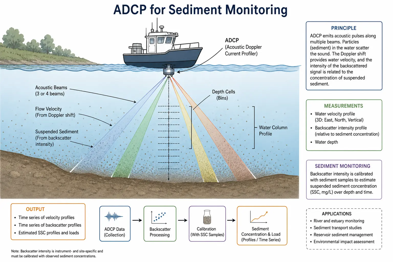
An ADCP transmits pulses of sound into the water and listens for the echo. Most people know it measures water velocity from the Doppler shift of that echo. Fewer realise the same echo carries information about the concentration and size of particles suspended in the water — the sediment.
2.1 The Acoustic Backscatter Principle
When an ADCP’s acoustic pulse encounters particles in the water column — sediment grains, plankton, bubbles — a fraction of the sound energy is scattered back toward the transducer. The strength of this returned signal is the acoustic backscatter intensity, measured in decibels (dB).
The key relationship is:
Higher sediment concentration → Stronger backscatter → Higher recorded echo intensity
But it is not a simple one-to-one relationship. The backscatter strength depends on three things simultaneously:
- Sediment concentration (SSC) — More particles mean more scatterers, so more energy returns. This is the relationship we want to calibrate.
- Particle size — For a given concentration, a single 200-micron sand grain scatters far more energy than the same mass distributed across thousands of 10-micron silt particles. This is why grain size matters enormously in acoustic sediment monitoring.
- Sound attenuation — As the acoustic pulse travels through sediment-laden water, it loses energy both to geometric spreading and to absorption and scattering by the sediment itself. This attenuation must be corrected for, or the ADCP will systematically underestimate sediment concentration at greater ranges.
The standard form of the sonar equation applied to ADCP sediment monitoring, following the approach developed by Gartner (2004) and Deines (1999), is:
10 log10(SSC) = A + B × (E − Er)
Where SSC is suspended sediment concentration (mg/L), A and B are empirically calibrated coefficients for a given frequency and grain size distribution, E is the echo intensity measured by the ADCP, and Er is the reference echo intensity. The coefficients A and B are not universal — they must be determined by collecting physical water samples alongside ADCP measurements and performing a linear regression.
2.2 Frequency Selection for Sediment Monitoring
The ADCP’s operating frequency determines what sediment sizes it is sensitive to. The physics is governed by the ratio of acoustic wavelength to particle circumference — the ka value, where k = 2π/λ (the acoustic wavenumber) and a is the particle radius:
- Rayleigh regime (ka ≪ 1): When particles are much smaller than the wavelength, backscatter increases with the fourth power of frequency. Fine silt and clay fall into this regime for most ADCP frequencies.
- Geometric regime (ka ≫ 1): When particles are much larger than the wavelength, backscatter becomes independent of frequency and proportional to the particle’s cross-sectional area. Coarse sand and gravel fall here.
- Mie regime (ka ≈ 0.5–10): The transition zone, where the relationship is complex and oscillatory. Medium silt to fine sand often occupies this range for common ADCP frequencies.
Here is how common ADCP frequencies map to sediment monitoring sensitivity:
| ADCP Frequency | Wavelength | Most Sensitive To | Typical Depth Range | Best Sediment Monitoring Application |
|---|---|---|---|---|
| 1200 kHz | ~1.25 mm | Fine silt to fine sand (10–200 μm) | 0.2–25 m | Shallow streams, laboratory flumes, irrigation canals |
| 600 kHz | ~2.5 mm | Medium silt to medium sand (30–500 μm) | 0.8–75 m | Medium rivers, reservoir delta monitoring, flood sediment pulses |
| 300 kHz | ~5.0 mm | Coarse silt to coarse sand (60–1000 μm) | 1–150 m | Large rivers, estuarine turbidity maxima, coastal sediment plumes |
| 75 kHz | ~20 mm | Fine sand to gravel (>200 μm) | 10–600 m | Deep-water sediment plumes, dredging impact monitoring, canyon flows |
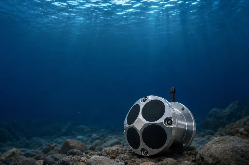
The 600 kHz sweet spot for sediment monitoring. For the majority of river and estuary sediment monitoring programmes, a 600 kHz ADCP strikes the best balance. It is sensitive to the silt and fine sand that make up the bulk of suspended sediment transport in most rivers, it profiles deep enough for all but the largest channels, and its cell size (typically 0.5–1.0 m) gives adequate vertical resolution of the sediment concentration profile. The Oceantek ADCP-600-SC-FA4 is a self-contained 600 kHz instrument purpose-built for this kind of long-duration sediment monitoring deployment, with titanium transducer housing that resists abrasion from sediment-laden flows.
3. From Echo Intensity to Sediment Concentration: The Calibration Process
An ADCP does not measure sediment concentration directly. It measures echo intensity. Converting echo intensity to suspended sediment concentration (SSC) requires a site-specific calibration. This is the single most important step in any ADCP sediment monitoring programme, and the one most frequently done poorly.
3.1 Water Sample Collection
Calibration requires paired measurements: ADCP backscatter data and physical water samples collected at the same time and location. The standard approach is:
- Mount the ADCP on a survey vessel or fixed platform and record echo intensity profiles.
- Simultaneously collect depth-integrated or point-integrated water samples using a calibrated sampler (e.g., US D-74, P-61, or a pumped sampling system).
- Filter each sample through pre-weighed 0.45 μm filters, dry, and re-weigh to determine SSC gravimetrically.
- Repeat across a range of flow conditions — low flow, moderate flow, and at least one flood event if possible. A minimum of 20–30 paired samples spanning the expected SSC range is recommended.
3.2 Correcting for Transmission Losses
Before fitting the calibration regression, the raw echo intensity must be corrected for sound attenuation along the acoustic path. Two corrections are essential:
- Geometric spreading loss: Sound intensity falls off with the square of distance from the transducer. In decibel terms, this is a 20 log10(R) correction, where R is slant range, plus a near-field correction for ranges within the transducer’s Fresnel zone.
- Water and sediment attenuation: Sound is absorbed by water itself (a function of temperature, salinity, and frequency) and additionally attenuated by the suspended sediment the pulse travels through. The sediment attenuation term is iterative — you need to know SSC to correct for its attenuation, but you need the attenuation correction to calculate SSC. Modern processing routines solve this by iterating until convergence.
Most ADCP manufacturers provide software that handles these corrections. The Oceantek ADCP-600-DR-FA4 outputs corrected backscatter in its standard PD0 data format, making it directly compatible with third-party sediment processing software such as the USGS Sediment Acoustic Leadership Team (SALT) toolbox and the USACE Sediment Analysis Suite.
3.3 Building the Calibration Curve
With corrected backscatter and measured SSC values in hand, a linear regression is fitted in log-space:
log10(SSC) = A + B × RB
Where RB is the relative backscatter (range-corrected and water-attenuation-corrected echo intensity). The slope B and intercept A are site-specific and, critically, grain-size-specific. If the grain size distribution changes significantly between low flow and flood flow — as it often does — a single calibration may not be valid across all conditions. A more sophisticated approach uses multi-frequency ADCP data to account for changing grain size, but this remains an active area of research.
4. Deployment Strategies for Sediment Monitoring
Different sediment monitoring objectives call for different ADCP deployment configurations. Here are the four most common strategies and when to use each.
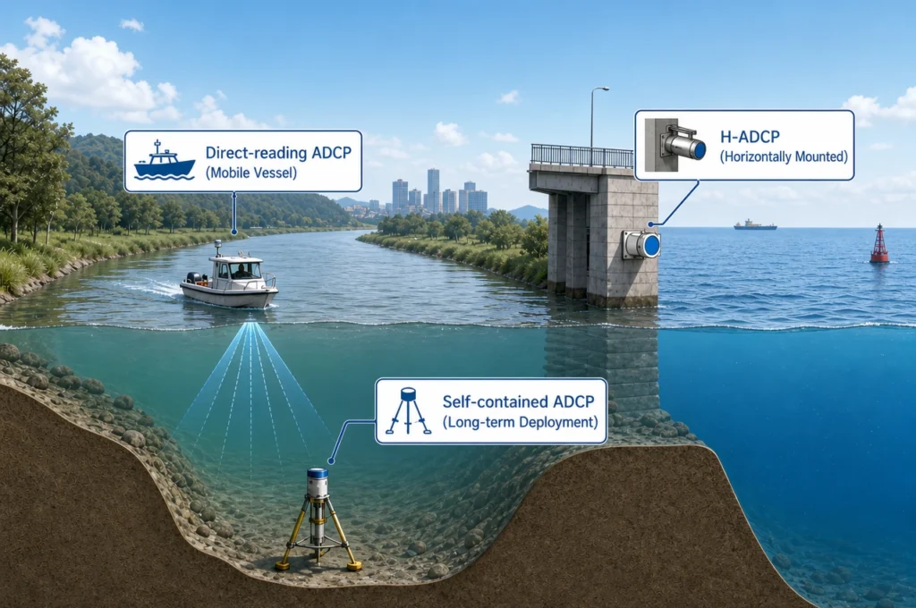
4.1 Moving-Boat Transects (Spatial Surveys)
The ADCP is mounted on a survey vessel that crosses the river from bank to bank. Each transect captures the full lateral and vertical distribution of velocity and backscatter. This method answers the question: how is sediment distributed across the channel right now? It is ideal for:
- Mapping sediment concentration cross-sections at a gauging station
- Quantifying lateral variability in sediment flux
- Calibrating index-velocity sediment rating curves
- Surveying reservoir delta progression
For medium-to-large rivers, a 600 kHz instrument with robust bottom tracking is the standard choice. The Oceantek River-ADCP-M9 is designed specifically for moving-boat discharge and sediment transects, with a compact hull that minimises flow disturbance and a ninth vertical beam for independent sediment concentration verification.
4.2 Fixed Horizontal ADCP (Continuous Monitoring)
A horizontal ADCP (H-ADCP) is mounted on a riverbank or bridge pier, aimed horizontally across the flow. It measures a single horizontal slice of velocity and backscatter continuously — 24 hours a day, 365 days a year. This is the only practical way to capture sediment dynamics during flood events, which often occur at night and may last only a few hours.
The Oceantek HADCP-600 is a purpose-built horizontal ADCP for permanent sediment monitoring installations. Its titanium housing withstands prolonged immersion in abrasive, sediment-laden water, and its low power consumption allows solar-powered operation at remote sites. Combined with cellular or satellite telemetry, it delivers real-time sediment flux data directly to the monitoring agency’s database.
4.3 Moored Upward-Looking Deployment
An ADCP is deployed on the seabed or riverbed, looking upward. This configuration captures the vertical structure of sediment concentration through the full water column and is widely used for:
- Long-term sediment flux monitoring at a fixed cross-section
- Shelf and coastal sediment transport studies
- Dredging plume monitoring
- Deep-water sediment gravity flow detection
The Oceantek ADCP-300-SC-FA4 is a 300 kHz self-contained ADCP optimised for moored sediment monitoring. Its high-capacity internal storage (up to 32 GB) and low-power design support deployments of six months or longer — enough to capture an entire flood season without servicing.
4.4 Vessel-Mounted Profiling (Deep Water)
For coastal and offshore sediment monitoring — dredge plume tracking, river plume dispersion, submarine canyon flows — a lower-frequency ADCP is required to penetrate to greater depths. The Oceantek ADCP-75-DR-PA4, a 75 kHz phased-array instrument, profiles to 600 metres and is sensitive to the sand-sized particles that dominate sediment transport in high-energy coastal environments. For platforms requiring bottom-lock in deep, turbid water — AUVs and ROVs operating in sediment-rich environments — the Oceantek DVL-600-PA5 provides rock-solid bottom tracking alongside current profiling, even through high suspended sediment loads.
5. Common Challenges in ADCP Sediment Monitoring
5.1 Changing Grain Size Distributions
The single biggest challenge in acoustic sediment monitoring is that the relationship between backscatter and concentration depends on particle size — and particle size changes with flow. During a flood, coarse sand that is normally immobile on the bed enters suspension, temporarily shifting the grain size distribution toward the coarser end. A calibration developed at low-to-moderate flow may underestimate SSC during floods because the coarser particles scatter more efficiently per unit mass. Multi-frequency approaches (e.g., simultaneous 600 kHz and 1200 kHz measurements) can help disentangle concentration and grain size effects, but they add complexity and cost.
5.2 Near-Bed Measurements
ADCPs have a blanking distance near the transducer face where meaningful backscatter data cannot be obtained. In a downward-looking vessel-mounted configuration, this means the near-bed region — often the zone of highest sediment concentration — is unmeasured. In an upward-looking moored deployment, the near-surface region is similarly lost. Side-lobe interference near the bed further contaminates the bottom 6–10% of the profile. Bedload transport, which can be a significant fraction of total sediment load in sand-bed rivers, is invisible to acoustic backscatter methods entirely.
5.3 High-Concentration Environments
At very high suspended sediment concentrations — above roughly 5,000–10,000 mg/L, depending on frequency — the acoustic signal is so strongly attenuated that the ADCP may lose bottom track or fail to profile at all. Hyperconcentrated flows, such as those in the Yellow River or during lahars, require alternative measurement techniques (e.g., pressure-difference samplers or nuclear densitometers).
5.4 Biofouling and Non-Sediment Scatterers
Acoustic backscatter does not distinguish between sediment particles and other scatterers — plankton, fish, bubbles, or flocculated organic matter. In biologically productive waters, especially during spring blooms, the backscatter signal may be dominated by zooplankton rather than sediment. In estuaries, flocculation — the aggregation of clay particles into larger, loosely bound flocs — changes the effective particle size and backscatter response without changing the total sediment mass. These effects must be understood and, where possible, accounted for in the monitoring programme design.
6. Best Practices for Reliable Sediment Monitoring Data
Drawing on guidelines from the USGS, ISO, and operational experience, the following practices will improve the quality and defensibility of ADCP-based sediment monitoring data:
- Calibrate with physical samples across the full flow range. A calibration developed from low-flow samples alone will not be valid at flood stage. Invest in sampling during at least one significant flow event per season.
- Collect grain size data alongside SSC samples. Knowing the particle size distribution for each calibration sample allows you to assess whether changes in the backscatter-SSC relationship are due to concentration changes or grain size shifts.
- Apply and document all corrections. Geometric spreading, water absorption, sediment attenuation, and near-field corrections all matter. Document which corrections were applied and with what parameters, so the data can be re-processed if methods improve.
- Use independent verification. An optical backscatter sensor (OBS) or laser diffraction instrument (LISST) deployed alongside the ADCP provides an independent check on sediment concentration that is not subject to the same acoustic ambiguities.
- Archive the raw backscatter data. Processed SSC values are only as good as the calibration. If the calibration is later found to be inadequate, the raw echo intensity data can be re-processed with an improved calibration — but only if it was saved in the first place. Always keep the manufacturer’s raw binary files.
- Match the frequency to the sediment and the site. A 1200 kHz instrument on the Amazon mainstem will not profile deep enough; a 75 kHz instrument in a 2-metre-deep stream will have blanking distances larger than the water column itself. Choose the frequency that matches your monitoring environment.
7. The Future of ADCP Sediment Monitoring
The technology continues to advance. Three developments deserve attention:
- Multi-frequency systems. Instruments that simultaneously transmit at two or more frequencies — such as 600 kHz and 1200 kHz from the same transducer head — provide information about both concentration and particle size by exploiting the different frequency responses of different size classes. This may reduce the dependence on physical calibration samples in the future.
- Real-time sediment flux reporting. Combined H-ADCP and telemetry systems are moving toward automated, near-real-time sediment flux calculations that feed directly into water resource management dashboards, giving operators timely data for reservoir flushing, diversion management, and environmental flow releases.
- Machine learning calibration. Researchers are using neural networks trained on large paired datasets of ADCP backscatter and physical SSC measurements to produce calibrations that generalise across sites and flow conditions — though the physics-based approach remains the standard for regulatory and scientific applications.
8. Choosing the Right Instrument for Your Sediment Monitoring Programme
The table below summarises the key instrument characteristics to consider when selecting an ADCP for sediment monitoring:
| Monitoring Scenario | Recommended Frequency | Deployment Mode | Key Consideration |
|---|---|---|---|
| Small river / stream (<5 m deep) | 600–1200 kHz | Moving-boat or wading | Fine vertical resolution needed in shallow water |
| Medium river (5–50 m deep) | 600 kHz | Moving-boat or fixed H-ADCP | Balance of penetration and sensitivity to silt/sand |
| Large river / estuary (50–150 m deep) | 300 kHz | Moving-boat or moored upward-looking | Need profiling range; coarser sediment typical |
| Reservoir sedimentation survey | 300–600 kHz | Moving-boat transects | Spatial mapping of delta progression |
| Continuous fixed-site monitoring | 600 kHz | Horizontal ADCP (H-ADCP) | Real-time data, flood capture, low power |
| Coastal / offshore sediment plume | 75–300 kHz | Vessel-mounted or moored | Deep profiling, sand transport dominance |
| Dredging impact monitoring | 300–600 kHz | Moored upward-looking array | Spatial coverage of sediment plume dispersion |
For comprehensive sediment monitoring solutions spanning river, estuarine, and coastal environments, Oceantek offers a full range of ADCP instruments from 75 kHz phased-array systems for deep-water sediment plume tracking to 600 kHz self-contained ADCPs for long-duration river sediment flux monitoring. Each instrument outputs industry-standard PD0 format data with corrected backscatter, compatible with USGS, USACE, and third-party sediment processing workflows.
Conclusion
ADCP-based sediment monitoring has moved from research technique to operational standard over the past two decades. The ability to measure velocity and suspended sediment concentration simultaneously — with the same instrument, on the same time base, across the full water column — provides a picture of sediment transport dynamics that physical sampling alone cannot match. The key to success is not the instrument itself but the calibration: paired physical samples collected across the full range of flow conditions, careful correction for acoustic transmission losses, and an honest assessment of the uncertainties introduced by changing grain size distributions. With these fundamentals in place, an ADCP becomes one of the most powerful tools available for understanding and managing sediment in rivers, reservoirs, estuaries, and coastal waters.
Whether you are establishing a new sediment monitoring programme or upgrading an existing one, choosing an instrument with robust backscatter output, reliable bottom tracking, and a transducer design that withstands abrasive sediment-laden environments is the foundation of quality data. Contact the Oceantek engineering team to discuss your sediment monitoring requirements and find the right ADCP configuration for your site.