Executive summary
The lowest metre of the water column is where bed friction, sediment transport and structure loading are decided, and it is the part of the profile that conventional ADCP configurations resolve least well. Measuring it is not a matter of selecting a finer cell size alone: the instrument's blanking distance and side-lobe interference set how close to the bed usable data can be obtained, and the processing mode determines whether centimetre cells are available at all. This guide explains the boundary layer structure worth resolving, the three constraints that govern a near-bed deployment, what can be derived from the resulting profile, and the configuration mistakes that most often invalidate the data.
Contents
- Why the lowest metre decides the physics
- What counts as near-bed: boundary layer structure
- The three constraints that govern a near-bed deployment
- Configuring an ADCP for near-bed work
- What you can derive from the profile
- Field checklist
- Common measurement errors
- Standards and uncertainty
- Frequently asked questions
- Conclusion
1. Why the lowest metre decides the physics
Almost everything that matters in coastal and river dynamics passes through the near-bed layer. Bed shear stress sets how much sediment can be entrained and how much drag a structure experiences. The velocity gradient in the lowest metre controls the vertical mixing that lifts sediment into the water column and keeps it there. Sediment flux — the product of concentration and velocity — is largest where both are large, which in most flows means the bottom few tens of centimetres.
It is also the hardest part of the profile to measure. A profiling ADCP placed on the seabed cannot see the water immediately above the transducer, and the cells closest to the bed are vulnerable to side-lobe interference. The result is a measurement gap where the processes of interest actually occur, and a set of derived quantities — bed shear stress, roughness length, flux — that depend on how well that gap has been handled.
2. What counts as near-bed: boundary layer structure
The bottom boundary layer is the region where friction at the bed has modified the flow. In shelf seas it is often one to ten metres thick; in rivers and estuaries it scales with depth and roughness. Within it, three zones matter for measurement design:
- The logarithmic layer — the lower ten to twenty percent of the boundary layer, where velocity varies logarithmically with height above the bed. This is the zone from which bed shear stress is normally estimated, and it is the primary measurement target.
- The roughness sublayer — the lowest centimetres to tens of centimetres, where individual roughness elements (gravel, ripples, vegetation) distort the flow and the log law does not apply.
- The wave boundary layer — in wave-influenced environments, a much thinner layer, centimetres to tens of centimetres thick, in which orbital velocities dominate the instantaneous flow.
The practical consequence is that a near-bed measurement programme is usually trying to resolve a layer between roughly 0.2 m and 2 m above the bed, at a resolution of centimetres to tens of centimetres, and it has to do so at heights where the instrument's own geometry and the bed's acoustic signature both interfere.
3. The three constraints that govern a near-bed deployment
3.1 Cell size
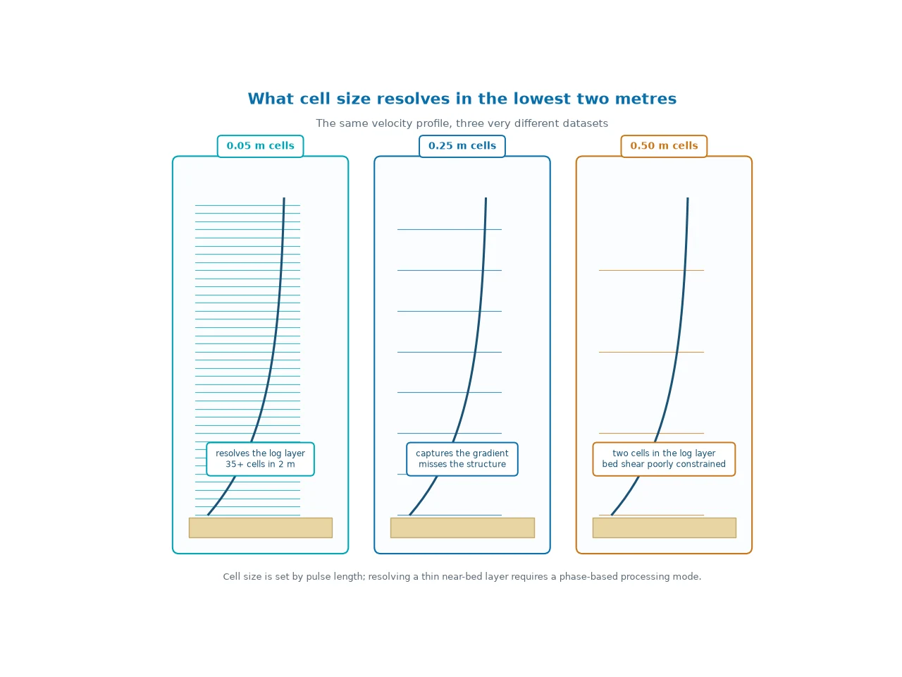
Resolving the log layer with enough cells to fit a profile requires cells of centimetres to a few tens of centimetres. Cell size follows pulse length, so this is a configuration decision, not an instrument class: it depends on the processing mode and on how much signal-to-noise ratio the site provides. Broadband cells of about 0.25 m and larger are usually too coarse for bed shear estimation, while a pulse-coherent configuration can produce cells of centimetres over a profile of a few metres. The trade-offs between modes are compared in our article on broadband and pulse-coherent processing, and the mechanism behind phase-based measurement is explained in the companion guide to pulse-coherent ADCP processing.
3.2 Blanking distance and side-lobe interference
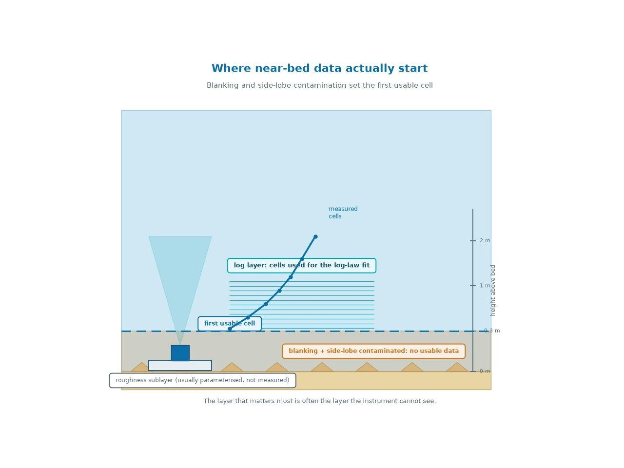
Two geometric limits determine how close to the bed a usable cell can sit. The blanking distance is the region immediately below the transducer where the instrument cannot receive during transmission; the first cell begins beyond it. Side-lobe interference occurs when energy returned from the boundary through the side lobes reaches the transducer before the main lobe has travelled to the bed, contaminating the lowest cells of the profile. There is no software fix for either limit — the affected cells are simply not usable.
Beam angle matters here. A wider beam angle increases the height band over which side-lobe contamination occurs, which reduces how close to the bed data can be obtained. This is one reason a narrow-beam piston design is often chosen for boundary layer work, even though a wider beam is more forgiving in rough terrain. The trade-offs between array geometries are compared in our article on 4-beam, 5-beam and 9-beam configurations.
3.3 Velocity range and mode limits
If the configuration uses pulse-coherent mode to obtain centimetre cells, the unambiguous velocity limit applies. Near-bed flows are usually slow, which is well matched to the method, but wave orbital velocities in the same layer can be several times the mean current. A site that looks suitable for a mean-flow measurement may exceed the velocity ceiling in the burst data. Checking the maximum instantaneous velocity, not just the tidal mean, is part of the deployment plan.
4. Configuring an ADCP for near-bed work
| Decision | Consideration | Typical practice |
|---|---|---|
| Processing mode | Centimetre cells require a phase-based method; range and velocity limits follow | Pulse-coherent for the boundary layer; broadband for the water column above it |
| Frequency | Sets wavelength, attainable cell size and attenuation | Higher frequency for fine cells at short range; see the frequency selection guide |
| Cell size | Must resolve the log layer; smaller cells reduce scatterers per cell | Centimetres to a few tens of centimetres, with averaging to control noise |
| Mounting height | First usable cell = blanking + cell + side-lobe standoff above the bed | Low frame, transducer clear of the bed and of scour |
| Sampling scheme | Wave bands need bursts; mean profiles need averaging | Bursts of minutes at 1 Hz or faster, repeated through the deployment |
| Beam geometry | Wider angles increase side-lobe contamination near the bed | Narrow beam angle where the lowest cells matter |
| Co-located sensors | Concentration and bed-level data are needed for flux and reference height | Optical or acoustic backscatter, plus an independent bed-level reference |
Mounting height is the decision that most often constrains the result. The transducer must clear the bed, avoid the scour it may generate itself, and stay below the layer of interest — three requirements that pull in different directions. A low-profile frame with the head a few tens of centimetres above the bed is the usual compromise, and the resulting first usable cell is often between 0.3 m and 1 m above the bed depending on blanking and beam angle. Frame and deployment options are covered in our guide to mounting solutions for buoys, tripods and fixed platforms, and the cell and range settings in ADCP configuration.
5. What you can derive from the profile
5.1 Bed shear stress from the log law
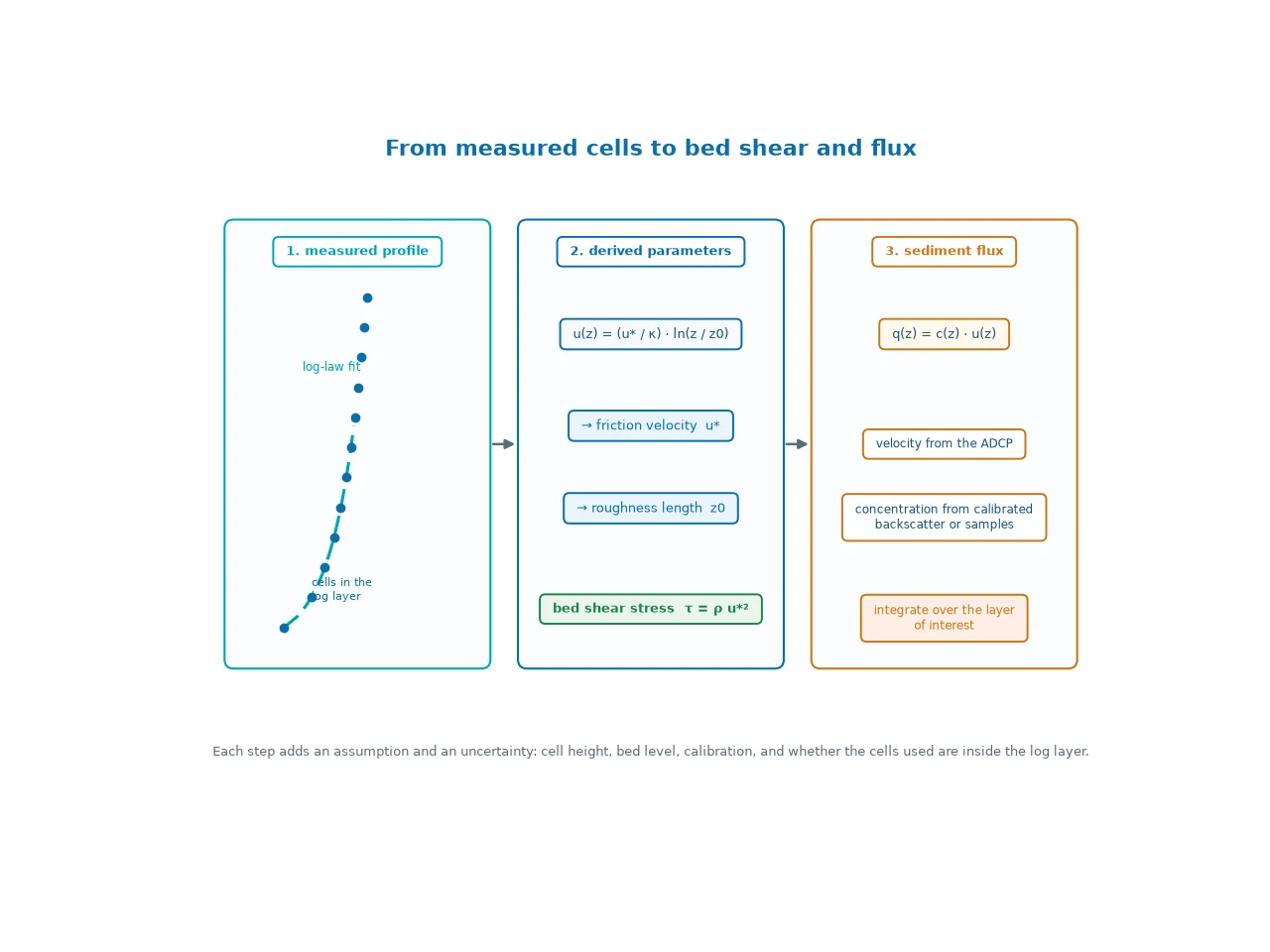
Inside the logarithmic layer, velocity varies with height above the bed as:
u(z) = (u* / κ) · ln(z / z0)
where u* is the friction velocity, κ is the von Kármán constant (about 0.4), z is height above the bed and z0 is the roughness length. Fitting this relation to the velocity cells inside the log layer yields u* and z0; bed shear stress follows as τ = ρ u*².
The fit is only as good as the input. It needs several cells inside the log layer, accurate cell heights above the bed, and assurance that the cells used are free of side-lobe contamination. Using cells from above the log layer, or using a bed level that drifted during the deployment, produces a friction velocity that looks plausible and is wrong.
5.2 Sediment flux
Sediment flux is the product of concentration and velocity, integrated over the layer of interest:
q(z) = c(z) · u(z)
An ADCP provides the velocity term and, through backscatter intensity, an indication of the concentration term. Converting backscatter to concentration requires site-specific calibration against water samples, because the relationship depends on grain size, density and the acoustic frequency. Once calibrated, fine near-bed cells make it possible to compute flux profiles rather than bulk estimates — which is the main reason boundary layer studies use them. The approach is described in our article on sediment monitoring with ADCPs.
5.3 Turbulence quantities
High-rate near-bed velocity data can be used to estimate turbulence characteristics such as Reynolds stress and turbulence intensity, provided the sampling rate, the noise level and the beam geometry support it. The assumptions are demanding — the flow field is assumed reasonably uniform across the beam spread — and the processing has to account for instrument tilt and wave bias. This is the application where pulse-coherent profilers are most often used, and where configuration errors are most visible in the results.
5.4 Wave-current interaction
Where waves are present, the near-bed velocity is the sum of a mean current and an oscillatory component. Separating them requires burst sampling fast enough to resolve the wave band, and the resulting estimates of bed shear normally distinguish wave, current and combined stress. Averaging a burst into a single mean velocity discards the information the deployment was designed to collect.
6. Field checklist
- Define the layer. State the height range to be resolved before choosing cells; the log layer, not the whole water column, is the target.
- Check the geometry. Calculate the first usable cell from blanking distance, cell size and side-lobe standoff, and confirm it falls below the top of the layer of interest.
- Match mode to requirement. Pulse-coherent for centimetre cells in slow flow; broadband for the column above; dual deployment when both are needed.
- Verify the velocity envelope. Use the maximum expected instantaneous velocity, including wave orbital motion, not the tidal mean.
- Plan the sampling scheme. Bursts for waves, averaging for means, and enough pings per average to control noise in thin cells.
- Record the bed level. An independent reference for bed height is needed to convert cell indices into heights above the bed, and it must be checked for scour or deposition during the deployment.
- Plan for biofouling and recovery. The lowest metre is also the most biologically active and the most exposed to sediment; service intervals follow.
7. Common measurement errors
7.1 Expecting the first cell at the bed
The profile starts below the transducer's blanking distance and above the side-lobe contaminated band. Deployments designed on the assumption that cell one sits at the bed produce a systematic offset in every derived height.
7.2 Using cells outside the log layer
Fitting the log law to cells that lie above the log layer yields a friction velocity that reflects the wrong flow regime. The layer has to be identified in the data, not assumed from the deployment depth.
7.3 Ignoring side-lobe contamination
Contaminated cells often look like valid data. The symptom is a profile that curves towards the bed in a way the log law does not predict; the check is to plot the profile against the fit and inspect the lowest cells.
7.4 Computing flux from a single velocity cell
Concentration and velocity both vary sharply near the bed, so flux computed from one cell ignores the structure that dominates the total. Fine cells exist to make the integration meaningful.
7.5 Averaging away the wave signal
A mean profile from a wave-influenced site is not a substitute for burst data. If the objective includes wave-driven stress, the sampling scheme has to resolve it.
7.6 Trusting an uncalibrated backscatter record
Backscatter intensity is a useful relative measure, but concentration requires calibration against samples from the site. Uncalibrated records are sometimes reported as concentrations; the resulting fluxes can be wrong by a large factor.
8. Standards and uncertainty
Near-bed measurement sits inside the same methodological framework as any other velocity-area or profiling measurement. ISO 24578 describes the moving-boat profiling case and the processing families, while the uncertainty framework in ISO 25377 (HUG) applies to derived quantities. That matters more here than in routine profiling, because bed shear stress and sediment flux are combinations of measured velocity, cell height, bed level and calibration coefficients, and each term carries its own uncertainty.
Where the deployment is part of a larger monitoring programme — a port, a dredging operation or an outfall — the near-bed record is usually interpreted alongside the wider current data. Two examples are covered in our articles on port and harbour monitoring and outfall monitoring.
9. Frequently asked questions
Can an ADCP measure velocity right at the seabed?
No. There is a blanking distance below the transducer and a band near the boundary where side-lobe returns contaminate the signal, so the first usable cell sits some distance above the bed. Its height depends on the instrument, the beam angle and the mounting height.
What cell size do I need for boundary layer work?
The log layer is roughly the lower ten to twenty percent of the boundary layer, so resolving it with several cells means cells of centimetres to a few tens of centimetres. Broadband cells of about 0.25 m and larger are usually too coarse for bed shear estimation.
How is bed shear stress calculated from ADCP data?
By fitting the logarithmic velocity profile to the cells inside the log layer, which yields the friction velocity. Bed shear stress is then the density multiplied by the square of the friction velocity.
Why does the beam angle matter near the bed?
Side-lobe energy can reach the boundary before the main beam, so the cells closest to the bed may be contaminated. A wider beam angle increases the affected height band and reduces how close to the bed usable data can be obtained.
Can an ADCP measure suspended sediment concentration?
Not directly. Backscatter intensity varies with suspended material, but conversion to concentration requires calibration against water samples from the site. Once calibrated, concentration multiplied by velocity gives a flux profile.
What sampling rate is needed for wave-dominated near-bed flow?
Wave orbital velocities vary on a scale of seconds, so burst sampling at about one hertz or faster is normal, with bursts repeated at intervals. Averaging suitable for a mean profile will smooth away the wave signal.
How low should the instrument be mounted?
Low enough that the first usable cell is inside the layer of interest, and high enough that the transducer clears the bed, moving sediment and any scour generated by the frame itself. That balance defines the frame design.
Are derived quantities like bed shear and flux uncertain?
Yes. Bed shear stress, roughness length and sediment flux combine measured velocity, cell heights, bed level and calibration terms, each with its own uncertainty. Where they are reported formally, the framework in ISO 25377 applies to the combination.
10. Conclusion
Near-bed measurement is a geometry problem as much as a resolution problem. The layer that matters is thin, the instrument cannot see the water immediately above it, and the cells closest to the bed are the ones most likely to be contaminated. Deployments that produce usable bed shear and flux data are the ones that state the target layer first, calculate the first usable cell before choosing a frame, and match the processing mode to the velocity range the site will actually produce — including the wave orbital velocities that a mean tide table does not show.
Published by Oceantek engineering team.Lasted update:September 24,2026.