Executive summary
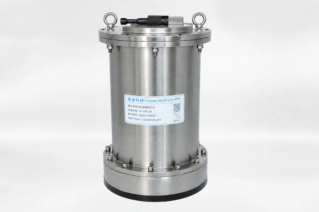
A 150 kHz acoustic Doppler current profiler sits between the mid-water instruments used in continental shelf and the low-frequency profilers used for full-depth ocean work. The Ocean-ADCP-150-PA4 profiles to 400 m, carries a pressure rating of up to 6,000 m and weighs 15.3 kg in air. This article explains what those specifications mean in practice, including how the ±1.0% ± 5 mm/s accuracy figure behaves at real flow speeds and where bottom tracking to 540 m helps.
Contents
- Where a 150 kHz instrument fits
- Profiling configuration: range, cells and layer thickness
- What the velocity accuracy figure means at your site
- Bottom tracking to 540 m
- Integrated sensors and why attitude correction matters
- Echo intensity as a second data stream
- Power, storage and integration
- Choosing the right pressure rating
- Typical applications
- Frequently asked questions
Where a 150 kHz instrument fits
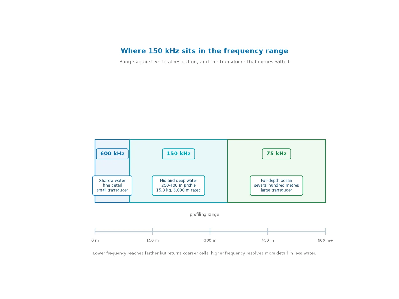
Frequency determines the basic trade-off in any Doppler profiler. A 600 kHz instrument resolves fine detail over tens of metres with a small transducer. A 75 kHz instrument reaches far into deep water, but the transducer becomes large and the depth cells coarse. A 150 kHz instrument occupies the middle of that range: 250 m to 400 m of profiling range in a housing that can be carried on a mooring, a seabed frame or an ROV. The underlying measurement principle is the same across the band, and is explained in our guide to how an acoustic Doppler current profiler works.
The transducer itself is a four-beam phased array with a 30° beam angle. Phased-array designs steer the acoustic beam electronically rather than tilting ceramic elements, which keeps the transducer face flat and the housing compact. Projects that only need nearshore coverage can use the smaller compact 600 kHz phased-array model instead.
That combination suits work on the continental shelf edge and upper slope, in deep channels, and in long-term moorings where the water column of interest extends well beyond the range of a 300 kHz or 600 kHz profiler. It also suits projects that need a ground-referenced velocity measurement at depths where a shallow-rated instrument cannot be deployed at all.
Profiling configuration: range, cells and layer thickness
| Parameter | Value |
|---|---|
| Operating frequency | 150 kHz |
| Transducer | Four-beam phased array, 30° beam angle |
| Operating modes | Broadband and pulse-coherent |
| Profiling range | 250 m / 400 m |
| Maximum number of cells | 255 |
| Cell thickness | 1–16 m (high precision); 4–16 m (long range) |
| Velocity accuracy | ±1.0% ± 5 mm/s typical |
| Velocity range | ±5.0 m/s default; expandable to ±10.0 m/s |
| Direction | 0–360°, accuracy ±2° |
| Bottom tracking | Up to 540 m |
| Echo intensity | 80 dB dynamic range, ±1.5 dB accuracy |
| Depth rating | 1,500 m / 3,000 m / 6,000 m |
| Housing | Titanium alloy |
| Size and mass | Φ215 × 318.9 mm excluding top connector; 15.3 kg in air |
The cell count and the cell thickness interact, and the 255-cell limit is the constraint that matters when a project wants fine resolution over a long range. A 1 m cell with the full 255 cells covers 255 m of the water column. A 4 m cell across 100 cells covers 400 m. Users who need both long range and fine resolution near a boundary normally configure a variable cell size, or accept a shorter profiling range for the fine-resolution part of the record.
Two operating modes are available. Broadband operation is the standard mode for general profiling. Pulse-coherent operation resolves smaller velocity differences over shorter ranges, which helps in quiet, weakly stratified water where the velocity signal is small. Choosing the mode is a site decision rather than a preference: it depends on the flow speeds and the vertical structure the project needs to capture. Two companion guides cover the wider decision: how to choose the right ADCP configuration and the key parameters to consider when selecting an ADCP.
What the velocity accuracy figure means at your site
The specified velocity accuracy is ±1.0% ± 5 mm/s. Both terms apply at the same time, and the fixed term matters most when the water is slow. At 1.0 m/s the combined error is about 15 mm/s, or 1.5% of the reading. At 0.2 m/s it is about 7 mm/s, or 3.5% of the reading. In deep, quiescent water, that difference is worth planning for, because a large part of the error budget comes from the fixed term rather than the flow itself.
The default velocity range is ±5.0 m/s, expandable to ±10.0 m/s. Most shelf and slope sites fall inside the default range, but tidal channels, straits and western boundary currents can exceed it, and the setting has to be checked against the site before deployment. Direction is resolved over 0–360° with ±2° accuracy, and the internal compass carries the same ±2° RMS specification. Because direction accuracy also depends on compass calibration and on setting magnetic declination correctly for the site, the specification is a starting point rather than the final number in the delivered data. Where a project has to report a formal uncertainty statement, the framework in ISO 25377 (HUG) shows how to combine the contributing terms.
Bottom tracking to 540 m
Bottom tracking measures velocity relative to the seabed instead of the water mass. With a maximum bottom-track depth of 540 m, the instrument can hold a ground reference in shelf and upper-slope settings that are far below the working depth of a 600 kHz profiler. On a moored or seabed-mounted instrument, bottom-track velocity indicates whether the bed itself is moving, which matters in sediment transport studies. On an ROV or a moving platform, the same measurement describes the motion of the platform.
Integrated sensors and why attitude correction matters
Temperature, pressure, tilt and heading are measured inside the instrument. Temperature covers -5 °C to 45 °C with ±0.1 °C accuracy and 0.03 °C resolution, which supports the sound-speed correction used in velocity processing. Pressure is specified at ±0.25% with 1 mm resolution, and in a bottom-mounted deployment it also provides a record of depth or water-level change. Tilt covers ±85° with ±0.3° RMS accuracy, and the compass covers 0–360° with ±2° RMS accuracy.
These measurements are not accessories. A mooring tilts with the current, and a seabed frame settles. Without tilt correction, the beam geometry assumed in processing no longer matches the instrument’s actual orientation, and near-surface or near-bed cells are the first to suffer. Heading correction is what allows velocity vectors from different instruments in the same array to be compared. A project that deploys several profilers should treat compass calibration as part of the survey design rather than as a post-processing step.
Echo intensity as a second data stream
The instrument records echo intensity across an 80 dB dynamic range with ±1.5 dB accuracy. Backscatter profiles are useful for tracking suspended matter and turbidity changes alongside the velocity record, and for identifying features that carry acoustic targets. Absolute concentration requires site-specific calibration against water samples, but relative changes over time and depth are available from the same deployment. For projects that would otherwise mount a separate backscatter sensor, this reduces the number of instruments on the frame and the number of cables in the water.
Power, storage and integration
Power input covers 20–50 V, and average consumption is 10 W or less. The arithmetic is straightforward for a deployment plan: a 1 kWh battery pack supports roughly 100 hours at 10 W average, so multi-month unattended deployments depend on duty cycling, larger packs or external power. On a moored or bottom-mounted frame, the practical approach is to define how often a profile is required and to size the pack against that duty cycle rather than against continuous operation.
Internal storage is 64 GB, which allows raw data to be retained on board through long deployments and reduces the risk of loss if a recovery is delayed. The communication interface supports RS-232 or RS-422, so the instrument connects to data loggers, mooring controllers and existing observation systems without a protocol conversion layer. The operating temperature range is -5 °C to 45 °C, and the instrument can be stored from -40 °C to 70 °C, which covers transport and laboratory storage between cruises.
Choosing the right pressure rating
Three depth ratings are offered: 1,500 m, 3,000 m and 6,000 m, all in a titanium housing. The rating should be chosen against the deepest point the instrument will reach, with an allowance for mooring knockdown and instrument tilt. Specifying the shallowest rating that covers the programme keeps mass and cost under control; specifying a 6,000 m instrument for a 1,200 m site adds capability the project will not use. Because the same transducer and electronics are used across the Ocean ADCP range, the choice of rating changes the housing, not the measurement performance.
Frame, mooring and platform mounting are covered in more detail in our guide to mounting solutions for buoys, tripods and fixed platforms.
Typical applications
- Deep-sea and continental slope research, where the water column of interest extends beyond the range of a 300 kHz profiler and the project needs velocity structure rather than a single point measurement.
- Subsea engineering and hydrological survey, including pipeline route and riser installation support, where current profiles inform installation windows and operational limits.
- Flow-field monitoring around oil and gas infrastructure, and metocean campaigns for offshore wind, where long-term records are needed at depths that rule out shallow-rated instruments.
- Long-term fixed-point ecological observation, where integrated temperature, pressure and backscatter data reduce the number of sensors that must be deployed alongside the profiler.
- ROV-deployed measurement campaigns, where a 15.3 kg instrument can be carried and positioned without a dedicated deployment frame.
Frequently asked questions
What does a 150 kHz ADCP measure?
It measures the velocity profile through the water column, together with flow direction, echo intensity, temperature, pressure, tilt and heading. The velocity profile is the primary output; the other measurements are used to correct and interpret it.
How far does a 150 kHz ADCP profile?
The Ocean-ADCP-150-PA4 is available in 250 m and 400 m profiling configurations with up to 255 depth cells. The practical range depends on cell thickness, the acoustic conditions of the site and the operating mode.
What is the velocity accuracy of the Ocean-ADCP-150-PA4?
Specified accuracy is ±1.0% ± 5 mm/s. At 1.0 m/s the combined error is about 15 mm/s; at 0.2 m/s it is about 7 mm/s, so the fixed term dominates at low flow speeds.
What is the difference between broadband and pulse-coherent modes?
Broadband operation is the standard profiling mode and covers the full range. Pulse-coherent operation resolves smaller velocity differences over shorter distances and is used in quiet water where the velocity signal is small.
Can it be deployed on a mooring, a seabed frame or an ROV?
Yes. The instrument weighs 15.3 kg in air and measures Φ215 × 318.9 mm excluding the top connector, and the three pressure ratings cover mooring, seabed and ROV deployments at different depths.
Does bottom tracking work at 540 m?
540 m is the maximum bottom-track depth. Whether the instrument holds bottom lock at a given site depends on the seabed type, the slope and the acoustic conditions, so the depth capability should be treated as an upper limit rather than a working guarantee.
Which pressure rating should I specify?
Choose the shallowest rating that covers the deepest point the instrument will reach, with an allowance for mooring knockdown and tilt. The 1,500 m, 3,000 m and 6,000 m versions share the same measurement performance.
This instrument is built for open water and deep deployments. For rivers, canals and inland channels, where a smaller profiler usually fits the section better, see our guide to water flow measurement.
Specifications quoted in this article are typical values for the Ocean-ADCP-150-PA4 and are provided for general guidance. Confirm figures for your configuration with our engineering team before specifying a system.