Executive Summary
A six-month project delay caused by insufficient current data can cost a wind farm developer tens of millions in re-design, re-consenting, and lost revenue. A properly designed ADCP measurement campaign, by contrast, represents less than 0.1% of total project capital expenditure.1
The arithmetic is straightforward. The execution is not.
This white paper provides a structured framework for planning an offshore wind current measurement campaign that satisfies financiers, insurers, and engineering teams alike. It covers:
- Where to measure — spatial coverage logic and deployment density recommendations
- How long to measure — minimum and best-practice durations by project phase
- What to measure — vertical profiling requirements and frequency selection
- How to ensure reliability — redundancy strategies and risk mitigation
- Instrument selection — a decision framework for ADCP frequency, deployment mode, and mooring configuration
- A 22-step campaign planning checklist — from desktop study to final data delivery
The guidance in this paper draws on lessons from metocean campaigns across North Sea, Irish Sea, and Asia-Pacific offshore wind projects, and reflects alignment with the IMarEST Metocean Procedures Guide (2024), DNV-ST-0437, and IEC 61400-3.
Oceantek provides ADCP and DVL instruments deployed in offshore wind measurement campaigns globally. This paper reflects practical experience from those deployments — it is not a sales document. Where Oceantek products are referenced, they appear because they match the technical requirements described, not the other way around.
1. Why Current Data Fails — And What It Costs
1.1 The Cost Asymmetry
Every offshore wind project measures wind. Not every project measures current with the rigour it deserves. When current data is absent, inadequate, or misinterpreted, the consequences propagate through design, construction, and operations — often silently until a failure occurs.
| Failure Mode | What Happens | Consequence | Order-of-Magnitude Cost |
|---|---|---|---|
| Current speeds underestimated | Foundation designed for lower lateral loads than reality | Foundation re-design post-FID; fabrication contract variation | $5M–$50M 1 |
| Current direction misaligned with wave direction | Combined wave-current load not captured in design basis | Cable burial depth insufficient; exposure and failure during storm | $2M–$10M per repair 2 |
| Insufficient seasonal coverage | Measurement campaign only captured summer low-current regime | Winter extremes missed; 50-year return period underestimated; insurer demands re-campaign | $500k–$2M repeat + insurance increase |
| Single-point measurement where profile was required | Current shear through water column not characterised | Foundation bending moment error of 15–30%; over-engineering or under-design | Missed cost-reduction or latent structural risk |
| Instrument failure during deployment | Data gap of 3–6 months before recovery possible | Campaign extension; financier questions data adequacy; delay to FID | $500k–$2M campaign repeat + delay |
| No real-time data during construction | Vessel operations proceed without current windows | Jack-up positioning incident; cable lay in unsafe cross-current; crane lift abort | $500k–$5M per incident 3 |
1 Industry estimate based on typical North Sea project data; foundation re-design costs vary widely depending on project scale and whether fabrication has already commenced.
2 Average export cable repair cost: $24 million (US/European data); average cable repair generally: €5 million per repair (2016 benchmark). Sources: GCube Insurance, international offshore engineering cost databases.
3 Industry estimate based on typical North Sea project data; individual incident costs vary significantly by vessel type and project phase.
1.2 The Regulatory Floor Is Not the Ceiling
Standards such as IEC 61400-3 (Design requirements for offshore wind turbines) and DNV-ST-0437 (Loads and site conditions for wind turbines) specify minimum metocean data requirements. These minima are designed to provide a baseline of safety and are periodically updated by technical committees.
They are not designed to satisfy project financiers or insurers.
Regulators specify what you must do. Financiers and insurers care about what you should do.
In practice, lender’s technical advisors (LTAs) and insurance underwriters increasingly expect current measurement campaigns that exceed regulatory minima:
| Parameter | Regulatory Minimum (Typical) | Lender / Insurer Expectation (Current Practice) |
|---|---|---|
| Measurement duration | 3 months (1 season) | 12 months minimum; 18–24 months preferred |
| Measurement locations | 1 location | 2–4 locations depending on site complexity |
| Vertical resolution | Single-point acceptable in some jurisdictions | Full water-column profile at all locations |
| Redundancy | Not specified | Minimum: staggered deployments; best practice: co-located pairs at critical locations |
| Data QC | Not prescribed | Full QA/QC protocol with documented flagging; NetCDF-CF compliant deliverables |
The gap between these two columns represents project risk. A campaign designed to the regulatory minimum leaves the developer exposed to LTA objections during due diligence, potentially delaying financial close by months.
1.3 The Insurance Perspective
GCube Insurance, the leading underwriter for renewable energy projects globally, published its decade-long analysis of offshore wind claims in the report “Uncharted Waters: Navigating Emerging Risks and Rising Claims in Global Offshore Wind” (covering 2010–2020). Key findings relevant to current measurement include:
- Subsea cables accounted for over 50% of total claims spend across the decade, with an average cable claim settlement of approximately £9 million.2
- 44% of cable claims spend was attributed to contractor error during transit and laying — much of which relates to operation in currents exceeding installation design assumptions.
- Total market losses from offshore wind claims reached £500 million by 2020, with average claim values nearly doubling from £1.67M (2010–2015) to £3.08M (by 2020).
- By 2021, GCube’s “Vertical Limit” report documented that average offshore wind losses had escalated further to over £7 million per claim.3
Not all cable claims are current-related. But current is a direct contributor to cable installation risk (cross-current during laying), burial adequacy (sediment mobility driven by near-bed currents), and long-term exposure (scour at cable crossings). An ADCP measurement campaign that properly characterises these currents is, in insurance terms, a risk mitigation measure — and is increasingly factored into underwriting decisions.
2. The Four Pillars of Campaign Design
Any metocean current measurement campaign for offshore wind can be evaluated against four dimensions. Weakness in any one pillar compromises the entire dataset — and, by extension, the engineering and financing decisions that depend on it.
| BANKABLE METOCEAN CURRENT DATASET | |||
|---|---|---|---|
| Pillar 1: Spatial Coverage How many locations? Where? | Pillar 2: Temporal Coverage How long do we measure? Which seasons? | Pillar 3: Vertical Coverage Which part of the water column matters? | Pillar 4: Reliability & Redundancy What happens if an instrument fails? |
Pillar 1: Spatial Coverage — How Many Locations and Where?
1a. The Logic of Spatial Sampling
You do not need an ADCP at every turbine location. But you do need enough spatial coverage to answer two fundamental questions:
- Is the current regime spatially uniform across the site, or does it vary significantly?
- If it varies, can the variability be characterised from a limited set of measurement points?
| Factor | How It Drives Spatial Variability | Examples |
|---|---|---|
| Bathymetric features | Sandbanks, channels, ridges, and troughs accelerate or funnel currents; tidal ellipse can rotate or amplify across a single sandwave field | Southern North Sea sandbank fields; Irish Sea troughs |
| Coastal proximity | Tidal amplification near headlands and in constricted channels; residual circulation driven by coastal geometry | Pentland Firth; English Channel approaches |
| Stratification | Seasonal thermoclines create decoupled surface and bottom current layers that may vary spatially depending on mixing | Summer-stratified North Sea sites; Baltic Sea |
| Regional circulation | Large-scale slope currents, oceanic inflows, or river plumes that interact with site-scale bathymetry | Norwegian Trench; Taiwan Strait; US East Coast Gulf Stream influence |
1b. Recommended Deployment Density
| Site Complexity | Typical Characteristics | Recommended ADCP Locations 1 | Example Regions |
|---|---|---|---|
| Low | Flat seabed (±5m), open water, weak tidal currents, well-mixed water column | 1–2 | Southern North Sea (uniform areas); Danish North Sea |
| Medium | Gentle slopes, moderate tidal range, some bathymetric features within 10km | 2–4 | Most UK North Sea sites; Irish Sea; German Bight |
| High | Complex bathymetry (sandbanks, channels), strong tides (>2 m/s), near headlands or in straits; stratified site | 3–6 | Pentland Firth; Taiwan Strait; Bay of Fundy; US East Coast shelf break |
1 Recommended ADCP locations are indicative. Final spatial layout should be informed by a site-specific hydrodynamic desktop study and, ideally, a preliminary model sensitivity analysis. Industry estimate based on typical North Sea project data.
1c. Placement Strategy
- Upstream/downstream pairs: Deploying two ADCPs along the dominant current axis captures how the current evolves as it crosses the site — invaluable for cable route characterisation.
- At proposed met mast / floating LiDAR locations: Co-locating current measurement with wind measurement de-risks two datasets simultaneously.
- Along the export cable route: At minimum, one ADCP should be positioned along the cable route at landfall, seabed transition zones, and cable crossing points.
- Avoid: placing the only ADCP in the lee of a sandbank, behind a headland, or in a known eddy zone — unless characterising that specific feature is the objective.
Pillar 2: Temporal Coverage — How Long to Measure?
2a. The Annual Cycle Problem
Currents in temperate shelf seas vary seasonally. Summer stratification can produce a two-layer flow regime that disappears in winter when the water column mixes. Storm-driven currents in winter can be two to three times stronger than mean summer currents.
If your measurement campaign only covers one season, you are not measuring the current regime — you are measuring one quarter of it.
At a North Sea site in ~45m water depth, a 3-month summer ADCP deployment recorded a mean near-surface current speed of 0.32 m/s, with a maximum recorded speed of 0.81 m/s. When the deployment was extended through winter (at the insistence of the LTA), the mean near-surface current rose to 0.68 m/s, and a storm event in January recorded a sustained current of 1.42 m/s at 10m depth — a value that would have been entirely missed by a summer-only campaign. The winter data changed the 50-year return period current estimate by approximately 35%, which in turn altered the foundation ultimate limit state design load and the scour protection specification.
Industry estimate based on typical North Sea project data; specific project data is confidential.
2b. Recommended Durations by Project Phase
| Project Phase | Minimum Acceptable | Best Practice | Rationale |
|---|---|---|---|
| Pre-FID / Feasibility | 3 months (1 season) | 12 months | Financiers demand full-year data before financial close; seasonal campaign acceptable for early screening only |
| FEED / Detailed Design | 12 months | 18–24 months | Enables robust extreme value analysis with reduced statistical uncertainty; captures inter-annual variability |
| Construction Support | Duration of construction (2–4 years) | Continuous real-time monitoring | Operational safety; current-window decision support for piling, cable laying, and heavy lifts |
| Operations (Scour Monitoring) | Continuous | Continuous with automated alerting | Scour is episodic — driven by storms. If you are not measuring during the storm, you miss the mechanism |
The IMarEST Metocean Procedures Guide (2024) notes that the primary driver of campaign duration is no longer technical feasibility but financier confidence. A single year of measured data, when combined with a validated multi-decadal hindcast model, is generally accepted as the minimum for financial close on projects in well-characterised regions such as the North Sea.6 For less-characterised regions (e.g., emerging Asian markets, US East Coast), 18–24 months is increasingly expected.
2c. Sampling Strategy Within the Deployment
| Parameter | Typical Configuration | Rationale |
|---|---|---|
| Ping rate | 1–2 Hz | Balances velocity precision against power consumption |
| Ensemble interval | 10–20 minutes | Standard for metocean characterisation; resolves tidal and subtidal variability |
| Saved profile interval | 10–60 minutes | Longer intervals reduce data volume without loss of relevant information |
| Bin size | 0.5m (600kHz), 1–2m (300kHz), 4–8m (75kHz) | Trade-off between vertical resolution and profiling range |
| Storm sampling | Triggered high-frequency mode | Increase sampling to 1–2 min ensembles when current/wave threshold exceeded |
Pillar 3: Vertical Coverage — What Part of the Water Column?
3a. Why a Full Profile Matters
Current is a vector that varies with depth. Current speed typically decreases toward the seabed (following a logarithmic or power-law shear profile), but stratification, internal waves, and bathymetric steering can produce complex profiles that a single-point measurement cannot capture.
A single-point current measurement at 5m depth, when used as a proxy for the full water column in a foundation bending moment calculation, can produce errors in the range of 15–30% compared to using a measured current profile.1
3b. What Matters at Each Depth Layer
| Depth Layer | What to Measure | Why It Matters | Engineering Application |
|---|---|---|---|
| Near-surface (top 20%) | Wind-driven current, wave-current interaction velocity | Rotor blade tip clearance; vessel access safety; floating platform station-keeping | Turbine design; O&M vessel operability limits; mooring system design |
| Mid-water (20%–80%) | Current shear profile; internal wave velocities; residual circulation | Dominant contributor to foundation bending moment and fatigue loading | Monopile/jacket structural design; fatigue life assessment |
| Near-bed (bottom 20%) | Bed shear stress; near-bed velocity; sediment mobility indicator | Scour potential; cable burial adequacy; foundation stability | Scour protection design; cable burial risk assessment; geotechnical integration |
For fixed-bottom turbines in 30–60m water depth — the majority of installed offshore wind capacity globally — a 300kHz ADCP provides full water-column profiling with 1–2m vertical resolution, capturing all three depth layers in a single instrument.
3c. ADCP Frequency and Vertical Coverage
| ADCP Frequency | Typical Max Profiling Range 1 | Typical Bin Size | Best-For Depth | Best Application |
|---|---|---|---|---|
| 600 kHz | 50–70 m | 0.5–1.0 m | <50 m | Shallow sites; high-resolution near-bed studies; cable landfall monitoring |
| 300 kHz | 100–150 m | 1.0–2.0 m | 30–120 m | Workhorse for most fixed-bottom offshore wind metocean campaigns |
| 75 kHz | 500–600 m | 4.0–8.0 m | >100 m | Deep-water floating wind; export cable routes on the continental shelf |
1 Typical range figures assume clear water and standard backscatter conditions. Actual range varies with water clarity, suspended sediment concentration, and instrument settings. For planning, use 70–80% of the stated maximum range as a conservative deployment envelope.
Pillar 4: Reliability — What Happens When an Instrument Fails?
4a. The Single-Point-of-Failure Problem
Consider this scenario: a developer deploys a single ADCP at a single location for a 12-month metocean campaign. At month 4, trawl damage severs the mooring. The ADCP is lost. The dataset — and the project’s current characterisation — is 33% complete.
The developer now faces:
- A 6–8 month gap before a replacement can be procured, permitted, and deployed
- An incomplete dataset that does not capture the full seasonal cycle
- A lender’s technical advisor who flags the data gap in the due diligence report
- Potential delay to financial close
The cost of in-water intervention — vessel mobilisation, ADCP procurement or rental, re-deployment — is in the range of $50k–$200k1 depending on location and instrument type. But the consequential cost of delayed FID dwarfs the intervention cost.
4b. Redundancy Strategies
| Strategy | Description | Cost Multiplier 1 | Risk Reduction | When to Use |
|---|---|---|---|---|
| Single instrument | One ADCP at one location | 1.0× (baseline) | 0% | Early-stage site screening; low-consequence campaigns |
| Staggered deployments | Two ADCPs deployed at different times (e.g., month 0 and month 2) | ~1.2× | ~40% | Budget-constrained; captures measurement gaps without doubling instruments |
| Spatial redundancy | ADCPs at separate locations with overlapping profiling ranges | ~1.5× | ~70% | Large, spatially coherent sites with gradual current variability |
| Co-located pair | Two ADCPs on the same frame, independently logging | ~1.8× | ~90% | Critical single-location deployments; high-consequence campaigns |
| Co-located pair + telemetry | Two ADCPs with surface buoy, alerting operators on failure | ~2.2× | ~95% | Highest-consequence; construction support; narrow FID windows |
1 Cost multipliers are indicative. Industry estimate based on typical North Sea project data. Actual costs vary with water depth, distance from port, and instrument configuration.
4c. The Insurance and Financing Implication
Lender’s technical advisors are increasingly asking two specific questions during due diligence:
- “What was your redundancy strategy for the current measurement campaign?”
- “What data gaps occurred, and how were they addressed?”
A documented redundancy plan — even a modest one such as staggered deployments — provides a defensible answer. In the current insurance market, where premiums for offshore wind construction have hardened considerably (GCube reports total market losses of £500 million by 2020, with average claims nearly doubling in five years2), demonstrating robust risk management in the measurement campaign can positively influence underwriting terms.
3. Instrument Selection Logic
3.1 Decision Framework
The following decision table provides a structured path from site characteristics to instrument recommendation.
| Water Depth | Condition | Answer | Recommended Instrument | Configuration & Notes |
|---|---|---|---|---|
| <30 m | Deployment >3 months? | Yes | Self-contained 600 kHz ADCP | Bottom-mounted frame, upward-looking. Bin size: 0.5–1.0 m |
| No | Direct-reading 600 kHz ADCP | Vessel-mounted or surface buoy telemetry. Real-time data; shorter deployment OK | ||
| 30–80 m | Real-time data required? | Yes | Direct-reading 300 kHz ADCP | Sub-surface buoy with surface telemetry, or seabed frame with telemetry buoy. Bin size: 1.0–2.0 m |
| No | Self-contained 300 kHz ADCP | Sub-surface taut-line mooring, or bottom frame upward-looking. Battery-powered; no surface expression | ||
| >80 m | Floating wind or deep cable route? | Yes | 75 kHz ADCP | Deep mooring configuration. Motion correction required. Bin size: 4.0–8.0 m |
| No | 300 kHz ADCP (if ≤150 m) | Taut-line mooring from seabed. Mid-water instrument depth |
The 300kHz ADCP is the workhorse for offshore wind metocean campaigns. Its profiling range (100–150m) covers the full water column at the 30–60m depths where most fixed-bottom turbines are installed.
3.2 Frequency Comparison: 600 kHz vs. 300 kHz vs. 75 kHz
| Parameter | 600 kHz | 300 kHz | 75 kHz |
|---|---|---|---|
| Typical max range | 55–70 m | 120–160 m | 550–650 m |
| Vertical resolution (bin size) | 0.5–4.0 m | 1.0–8.0 m | 4.0–32.0 m |
| Beam geometry | 4-beam, 20° Janus | 4-beam, 20° Janus | 4-beam or phased array, 30° |
| Velocity precision (per ping) 1 | ±0.3%–0.3 cm/s | ±0.5%–0.5 cm/s | ±1.0%–0.5 cm/s |
| Transducer diameter | ~150 mm | ~200–250 mm | ~300–400 mm (piston); ~200 mm (phased array) |
| Weight (in air, typical) | ~5 kg | ~10 kg | ~50kg |
| Deployment duration (self-contained) | 3–6 months | 6–12 months | 6–18 months |
| Relative equipment cost | $$ | $$$ | $$$$ |
| Best for offshore wind | Cable landfall; very shallow sites; high-resolution near-bed studies | Workhorse — most fixed-bottom turbine sites | Deep floating wind; export cable routes on continental shelf |
1 Ping-level precision. Ensemble-averaged precision improves with the square root of the number of pings per ensemble.
3.3 Direct-Reading vs. Self-Contained: The Real Trade-offs
| Factor | Direct-Reading | Self-Contained |
|---|---|---|
| Real-time data | Yes — data transmitted to shore/vessel | No — data retrieved on instrument recovery |
| Surface expression | Required (buoy, vessel, or platform) | None — fully submerged |
| Biofouling risk | Higher — buoy hull, cable, and surface expression attract growth | Lower — fully submerged; still requires anti-fouling for deployments >3 months |
| Vandalism / fishing risk | Higher — visible buoy attracts attention; mooring lines snag risk | Lower — submerged, unmarked; still vulnerable to bottom trawling |
| Storm vulnerability | Higher — surface buoy can break free or be damaged | Lower — fully submerged, no surface loads |
| Data continuity confidence | High — you know within hours if the instrument has failed | Unknown until recovery — a failed instrument at month 12 = 12 months lost |
| Power supply | Cable from surface (solar buoy, vessel, or shore) | Internal battery — must be sized for full deployment |
| Relative cost (full system) | Higher — buoy + cable + telemetry + power | Lower — instrument + frame + battery pack |
| Permitting complexity | Higher — navigation marking, lighting, Notices to Mariners | Lower — submerged, no surface navigation hazard |
| Best for | Construction support; critical single-instrument deployments | Long-term background monitoring; multi-instrument campaigns; high-traffic areas |
3.4 Mounting and Mooring Configurations
Three configurations cover most offshore wind ADCP deployment scenarios.
Configuration A: Bottom-Mounted Frame (Shallow Water, Upward-Looking)
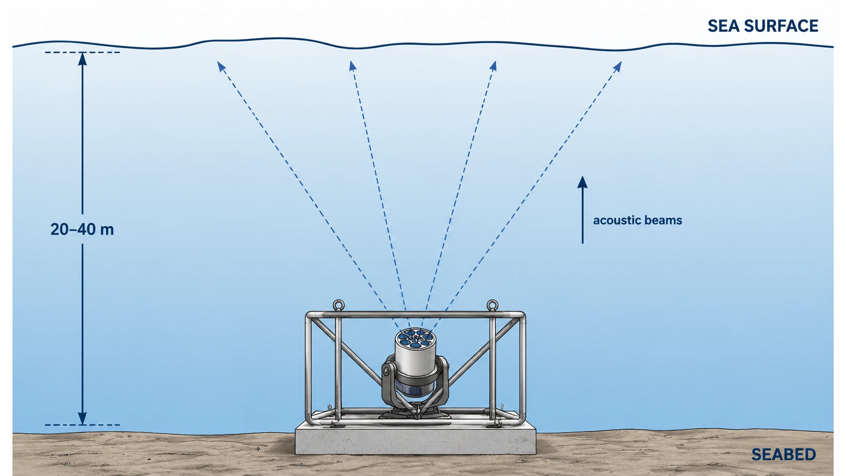
Best for: Water depths ≤50m; self-contained deployments of 3–12 months.
Key considerations: Frame must resist current drag and trawl snag loads. Gimbal mount maintains ADCP within pitch/roll tolerance (±15°). Acoustic release on the frame enables recovery without diver intervention.
Configuration B: Sub-Surface Taut-Line Mooring (Mid-Depth)
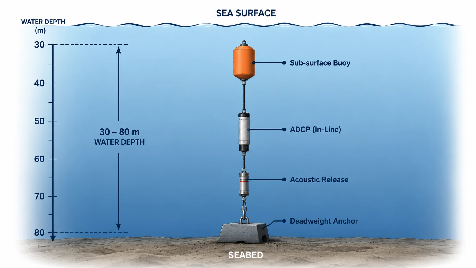
Best for: Water depths 30–80m; deployments where surface expression is undesirable.
Key considerations: Sub-surface buoy must be deep enough to avoid vessel interaction (5–10m below surface in North Sea). Taut-line minimises instrument motion but motion correction should still be applied in post-processing.
Configuration C: Seabed Frame with Surface Telemetry Buoy (Real-Time)
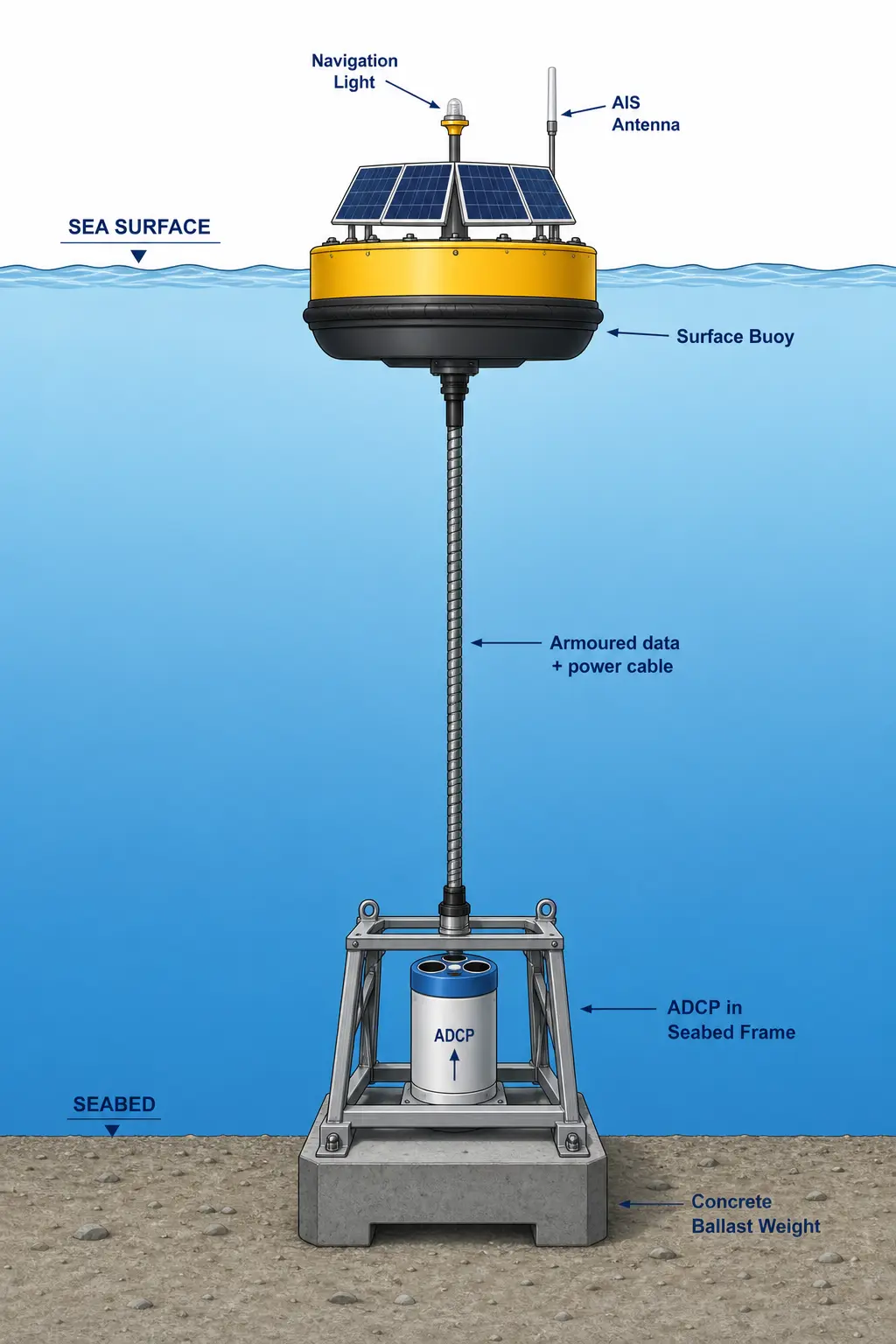
Best for: Any depth where real-time data is required; construction support; critical single-point deployments.
Key considerations: The cable is the single most vulnerable component — must be armoured and, in high-traffic areas, buried. Buoy requires periodic maintenance (solar panel cleaning, navigation light checks). Highest-cost configuration.
4. Data Management and Deliverables
4.1 What the End User Actually Needs
The developer and their engineering team do not need raw beam velocities in proprietary binary format. They need actionable, quality-controlled data products:
| ADCP Records | Processing Step | Client Receives |
|---|---|---|
| Beam velocities (4 beams × N bins × M ensembles) | Coordinate transformation (beam → Earth) | East / North / Up velocity components |
| Correlation magnitude (per beam, per bin) | QC screening threshold | Flagged data: good / suspect / bad |
| Echo intensity (per beam, per bin) | Profile review | Biofouling / sediment layer diagnostic |
| Temperature, pressure, pitch, roll | Sensor health QC | Instrument health summary; deployment metadata |
| Bottom-track velocity | BT QC; comparison with GPS (if available) | Vessel-referenced or Earth-referenced current |
4.2 QA/QC Protocol
| QC Parameter | Check Method | Typical Threshold | Action on Failure |
|---|---|---|---|
| Correlation magnitude | Per-beam, per-bin | >64 counts (TRDI-style) | Flag bin; cross-reference with echo intensity |
| Percent good | Per-bin | >80% for ≥3 of 4 beams | Flag bin; if persistent, investigate instrument health |
| Pitch / Roll | Per-ensemble sensor check | Pitch ±15°; Roll ±15° | Flag ensemble; if persistent, review mooring |
| Velocity spike | Temporal gradient check | >1.0 m/s change between adjacent ensembles | Flag ensemble; review for real event vs. artefact |
| Echo intensity | Profile inspection | Sudden unexplained drop; significant beam asymmetry | Investigate biofouling, sediment plume, or transducer damage |
| Side-lobe interference | Geometric calculation | Bottom 6% of range (20° Janus) | Flag as “side-lobe contaminated” — expected physical artefact |
| Temperature / Pressure | Compare vs. bench test and CTD cast | Deviation >0.5°C or >1% pressure | Cross-reference with independent sensor; may need re-calibration |
4.3 Deliverable Formats
| Format | Purpose | Standard |
|---|---|---|
| NetCDF-CF | Primary archival format; machine-readable; self-describing metadata | CF Conventions 1.8+ with OceanSITES attributes |
| CSV | Quick inspection; Excel import for non-specialist review | UTF-8, ISO 8601 timestamps, header rows with variable names and units |
| MATLAB .mat | Engineering team ingest; integration with hydrodynamic model pipeline | Version 7.3; structure array with time, depth, u, v, w |
| QC report (PDF) | Client-facing summary of data quality, rejection rates, instrument health | Documented flag definitions; per-instrument summary statistics |
5. Budget and Value
5.1 Order-of-Magnitude Campaign Costs
| Campaign Scale | Instruments | Duration | Indicative Cost Range 1 | As % of Total Project CAPEX 2 |
|---|---|---|---|---|
| Minimum viable | 1 | 3 months (1 season) | $60k–$120k | <0.02% |
| Industry standard | 2–3 | 12 months | $200k–$450k | <0.05% |
| Best practice | 3–6 | 18–24 months | $400k–$900k | <0.10% |
1 Industry estimate based on typical North Sea project data. Cost components include: ADCP instrument (procurement or rental), mooring/frame hardware, vessel days for deployment and recovery (CTV day rates in the range €5,500–€8,000 as of 2024–2025; source: Clarksons offshore vessel index and publicly disclosed Baltic tender data4), data processing and reporting, and contingency. Actual costs vary significantly with water depth, distance from port, and local vessel market conditions.
2 Based on total development CAPEX for a typical 500MW–1GW offshore wind project. Full metocean data & monitoring is estimated at approximately 0.5% of CAPEX (source: Atkins, 20185); the ADCP current measurement component is a subset of this.
Cost drivers in descending order of impact:
- Number of deployment locations and instruments
- Vessel day rates (highly region-dependent; North Sea higher than SE Asia)
- Direct-reading vs. self-contained (real-time telemetry adds approximately 40–80% to per-location cost)
- Deployment duration (incremental cost per additional month is primarily data processing)
- Redundancy strategy (staggered deployments: ~+20%; co-located pairs: ~+80%)
5.2 The Value Equation
The value of a properly designed ADCP campaign is not in the data — it is in the avoided cost of decisions made on the basis of inadequate data:
| Cost of… | Indicative Magnitude | Source |
|---|---|---|
| A best-practice ADCP measurement campaign (3–6 instruments, 18–24 months) | $400k–$900k | Industry estimate 1 |
| A single export cable repair | $24 million (average) | US / European offshore wind data |
| A single cable insurance claim settlement | ~£9 million (average) | GCube Insurance, 2010–2020 2 |
| A foundation re-design after fabrication has commenced | $5M–$50M | Industry estimate 1 |
| A 6-month delay to financial close | $10M–$50M+ | Project finance industry benchmarks |
1 Industry estimate based on typical North Sea project data.
2 Source: GCube Insurance, “Uncharted Waters” (2020). Headline statistics publicly reported via Windpower Engineering, EnergyPeople, and Modern Power Systems.
The ratio is 5:1 to 50:1 in favour of the measurement campaign. The cost of the ADCP campaign, when expressed as a percentage of total project CAPEX, rounds to zero. When viewed against the cost of getting the current regime wrong, it is one of the highest-return risk-mitigation investments available in the pre-FID phase.
6. Campaign Planning Checklist
The following 22-step checklist is designed as a standalone planning tool.
Pre-Deployment (Steps 1–10)
- [ ] Define data requirements. Document which current parameters are required, at what depths, to what accuracy, and which engineering decisions they feed into.
- [ ] Complete a hydrodynamic desktop study. Review existing current data: regional tidal models, nearby measurement campaigns, tidal atlases, satellite altimetry.
- [ ] Run a preliminary model sensitivity analysis (if available) to identify areas of greatest current uncertainty — these are your priority measurement locations.
- [ ] Determine the number of ADCP locations using the complexity framework in Section 2, Pillar 1.
- [ ] Determine deployment duration per location using the phase-based recommendations in Section 2, Pillar 2.
- [ ] Select ADCP frequency and configuration per location using the decision framework in Section 3.
- [ ] Design moorings/frames for each deployment location. Ensure adequate ballast for the expected current regime.
- [ ] Prepare a redundancy plan. Document the chosen strategy, the contingency budget, and the trigger criteria for invoking contingency.
- [ ] Bench-test all instruments: ping test, pressure test, clock sync, battery voltage, data download test, configuration file backup.
- [ ] Obtain all required permits: marine licence, Notice to Mariners, navigation marking approval, fisheries liaison.
Deployment (Steps 11–14)
- [ ] Record deployment metadata: exact position (DGPS), orientation (heading), water depth, time of first ping, instrument serial number, configuration file, battery voltage at deployment.
- [ ] Verify data return: For real-time systems, confirm data receipt and quality within 48 hours. For self-contained, conduct diver/ROV visual inspection within the first week if possible.
- [ ] Photograph everything: frame on deck, instrument in frame, deployment over the side, surface buoy (if used), DGPS display with coordinates.
- [ ] File a deployment report within one week: all metadata, photographs, and any deviations from the deployment plan.
During Campaign (Steps 15–18)
- [ ] Daily QC check (real-time systems): review for correlation drop, velocity spikes, pitch/roll excursions, echo intensity anomalies.
- [ ] Mid-campaign service visit (for deployments ≥6 months): clean transducer face and buoy hull, check battery, download partial dataset, inspect mooring.
- [ ] Monitor for external threats: fishing activity, storm track forecasts, AIS position (surface buoys) during storm season.
- [ ] Maintain a campaign logbook: service visits, storm passages, anomalies, communications with fisheries or maritime authorities, configuration changes.
Recovery and Processing (Steps 19–21)
- [ ] Recover instruments safely: confirm acoustic release function; download data immediately; photograph instrument condition before cleaning.
- [ ] Run the full QC processing pipeline using the protocol in Section 4.2. Document all QC decisions. If data rejection exceeds 10–15% in any depth bin, investigate and document the cause.
- [ ] Generate deliverables package: QC’d dataset in NetCDF-CF, statistical summary, current rose, extreme value analysis (1-year, 50-year), time series plots, QC report.
Post-Campaign (Step 22)
- [ ] Archive everything: raw binary data, processed NetCDF files, configuration files, logbook, deployment/recovery reports, QC report, photographs. Store in at least two physically separate locations.
7. Conclusion
Current data quality determines design certainty. Design certainty determines financial close. The relationship is direct: the more confidence you have in your understanding of the current regime, the less contingency — in steel tonnage, in insurance premiums, in financing margins — you carry through the project lifecycle.
A well-planned ADCP measurement campaign is the cheapest insurance a wind farm developer can buy. Its cost is a rounding error in the project CAPEX. The cost of not doing it properly can be measured in tens of millions.
The framework in this paper — four pillars of campaign design, a structured instrument selection logic, a documented QC protocol, and a 22-step checklist — is designed to be applied directly. It reflects lessons from metocean campaigns in the North Sea, the Irish Sea, the Taiwan Strait, and beyond. Follow it, and your current dataset will withstand scrutiny from engineers, lenders, insurers, and regulators alike.
Next Steps
- Discuss your campaign with our engineers: Contact Oceantek
- View the ADCP Product lines: ADCP Products
Appendix A: Glossary
| Term | Definition |
|---|---|
| ADCP | Acoustic Doppler Current Profiler — measures water current velocities across a vertical profile using Doppler shift of acoustic signals |
| Bin | A depth cell — the vertical segment of the water column within which the ADCP averages velocity |
| Blanking distance | The zone immediately in front of the transducer where velocity cannot be reliably measured (typically 0.5–2.0m) |
| CAPEX | Capital expenditure |
| CF Conventions | Climate and Forecast metadata conventions — a standard for describing Earth science data in NetCDF format |
| CTD | Conductivity, Temperature, Depth — oceanographic instrument used to validate ADCP sound speed assumptions |
| CTV | Crew Transfer Vessel — small vessel used to transport personnel to offshore installations |
| DVL | Doppler Velocity Log — ADCP optimised for underwater vehicle navigation, using bottom-track for velocity-over-ground |
| Ensemble | A single measurement cycle consisting of multiple pings averaged together |
| FID | Financial close / Final investment decision |
| FEED | Front-End Engineering Design |
| LTA | Lender’s Technical Advisor — independent consultant engaged by project financiers to review technical aspects |
| Metocean | Meteorology and oceanography — combined study of wind, wave, current, and water level conditions |
| NetCDF | Network Common Data Form — self-describing, machine-independent data format widely used in oceanography |
| Ping | A single acoustic transmission and reception cycle |
| QC | Quality control |
| Scour | Erosion of seabed sediment around a foundation or structure due to current and wave action |
| Side-lobe interference | Measurement artefact caused by acoustic energy reflecting off the seabed from a sidelobe rather than the main beam |
| SOV | Service Operation Vessel — larger vessel used for offshore wind O&M, serving as floating accommodation and logistics hub |
Appendix B: Key References
- IEC 61400-3 — Wind energy generation systems — Part 3: Design requirements for offshore wind turbines
- DNV-ST-0437 — Loads and site conditions for wind turbines (Det Norske Veritas)
- IMarEST — Metocean Procedures Guide for Offshore Wind (2024 edition). Institute of Marine Engineering, Science & Technology.
- Carbon Trust — Offshore Wind Accelerator (OWA): Floating LiDAR Recommended Practice
- GCube Insurance — Uncharted Waters (2020), and Vertical Limit (2023)
- OceanSITES — Data format and quality control reference manual for time-series oceanographic data
Appendix C: About Oceantek
Oceantek designs and manufactures acoustic Doppler current profilers (ADCPs) and Doppler velocity logs (DVLs) for oceanographic, hydrographic, and underwater navigation applications. Our product range spans 75kHz to 600kHz, in self-contained, direct-reading, and vessel-mounted configurations, deployed in metocean campaigns, offshore wind site assessments, port monitoring networks, and AUV/ROV navigation systems globally.
Contact: Oceantek Engineer Team
Footnotes
1 Industry estimate based on typical North Sea project data. Values are indicative and intended for campaign scoping purposes. Actual costs vary with site-specific conditions, vessel market rates, and regulatory requirements.
2 Source: GCube Insurance, “Uncharted Waters: Navigating Emerging Risks and Rising Claims in Global Offshore Wind” (2020). Headline statistics publicly reported via Windpower Engineering, EnergyPeople, and Modern Power Systems. Full proprietary dataset available to GCube insured clients and brokers.
3 Source: GCube Insurance, “Vertical Limit: When is bigger not better in offshore wind’s race to scale?” (2023). Publicly reported via industry media.
4 Source: Clarksons offshore vessel index, 2024–2025; Baltic Sea CTV contract data publicly disclosed by Polenergia/Equinor (October 2024) for the Bałtyk 2 and Bałtyk 3 offshore wind projects.
5 Source: Atkins, 2018 — “Friends of Floating: The Future’s Floating” cost breakdown analysis, cited in Carbon Trust / ORE Catapult Floating Wind Cost Reduction pathways.
6 Source: IMarEST Metocean Procedures Guide for Offshore Wind (2024). Available via IMarEST at imarest.org.
7 ADCP instrument pricing referenced from US EPA technical procurement documentation (2017) and industry market reports. Current manufacturer pricing available on request. Contact oceanadcp.com for current specifications and quotation.
Disclaimer: This white paper is provided for informational purposes. Project-specific engineering decisions should be supported by site-specific data and qualified professional judgement.