Executive summary
Two ADCPs with the same frequency, transducer and depth rating can return very different data, because the processing mode sets what the instrument can resolve. Broadband and pulse-coherent processing both use pulse pairs and phase information; the difference is whether the second pulse waits for the first echo to return. That single structural difference decides profiling range, cell size, the velocity ceiling and the noise you have to average away. This guide compares the two modes as measurement tools, gives a decision table by objective, and explains when a combined deployment is the better answer than choosing one mode.
Contents
- What the two modes share
- The one structural difference that explains the rest
- The operating envelope, compared
- Resolution: what cells you actually get
- Velocity range and ambiguity
- Which mode for which measurement
- Can one instrument do both?
- Configuration checklist
- Common mistakes
- What the standards say
- Frequently asked questions
- Conclusion
1. What the two modes share
Both broadband and pulse-coherent processing are Doppler methods. Both transmit acoustic pulses, receive echoes from particles moving with the water, and derive velocity from the change in the returned signal. Both rely on the echoes remaining correlated, and both are limited by the same physical conditions: signal-to-noise ratio, acoustic scattering, boundary interference and flow structure across the beam.
ISO 24578 groups ADCP signal processing into three families — pulse-incoherent, pulse-to-pulse coherent and broadband — and the distinction between the last two is structural rather than cosmetic. The mechanics of phase-based measurement are covered in our companion article on pulse-coherent ADCP processing; this article concentrates on the choice between modes.
It is worth separating two things that are often confused. Hardware determines the frequency, the transducer and the beams. The processing mode determines how the returned signal is turned into velocity, which cells are produced and what limits apply. Some instruments offer more than one mode on the same hardware, which means two datasets from the same instrument can have completely different envelopes. That is why the mode belongs in the deployment plan rather than in a menu chosen at the last minute.
2. The one structural difference that explains the rest
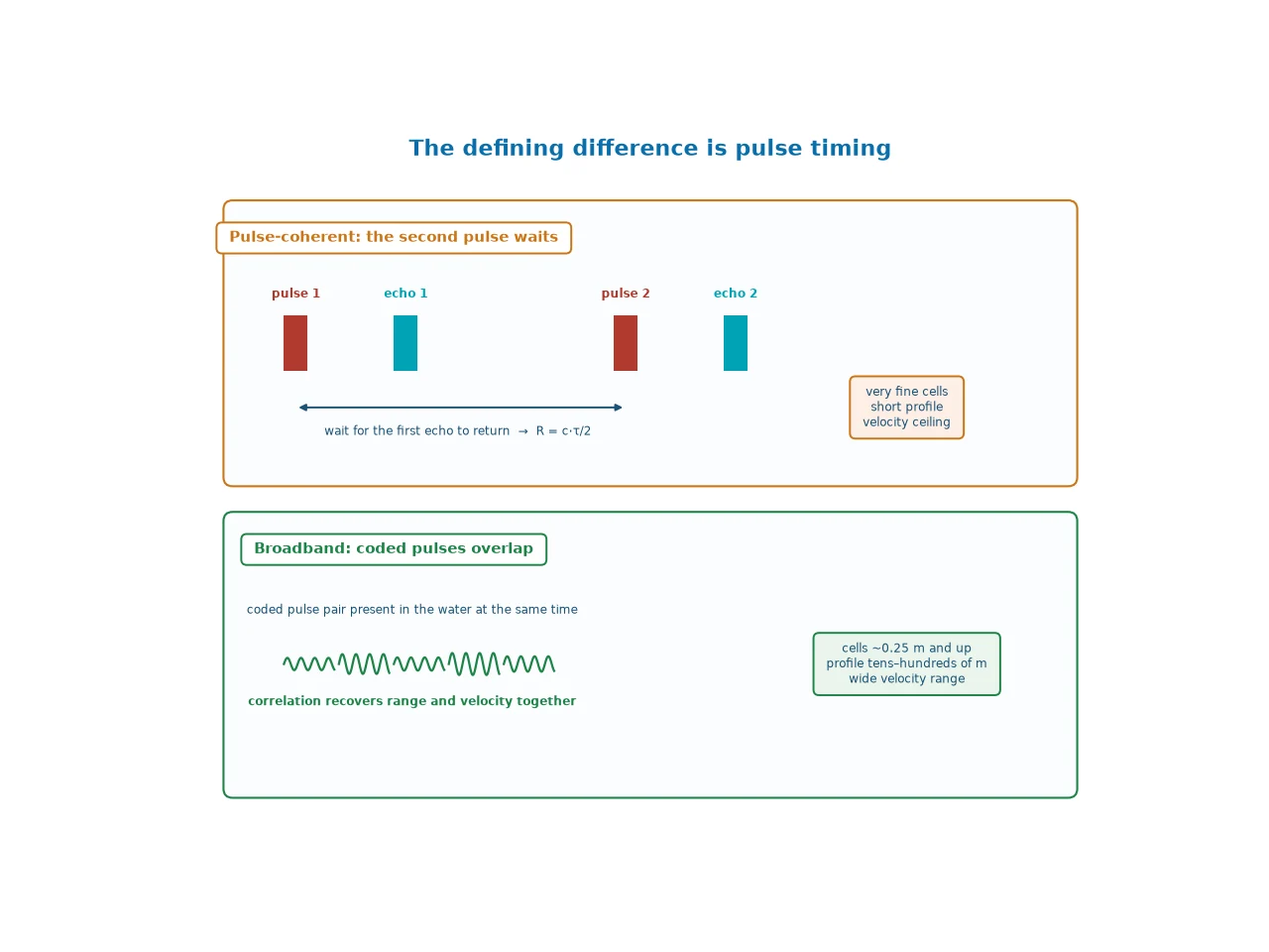
2.1 Pulse-coherent: the second pulse waits
In a pulse-coherent configuration the instrument transmits a short pulse, waits for the echo from the far end of the profile, and only then transmits the second pulse. That rule keeps the two echoes attributable to the same scattering volume, and it is what sets the maximum range:
Rmax ≈ c · τ / 2
Because the same lag τ also fixes the unambiguous velocity, V = λ / (4τ), range and velocity are coupled: the operating point sits on a fixed curve, and improving one degrades the other.
2.2 Broadband: coded pulses that overlap
A broadband system transmits coded pulses that can be present in the water at the same time. The received signal is correlated with the transmitted code, which separates returns by range while the phase difference between successive coded pulses provides velocity. The lag is no longer tied to the round-trip time to the far edge of the profile, so the range constraint is relaxed.
2.3 What that buys and what it costs
Broadband delivers a much longer profile and a far wider usable velocity range, at the cost of cell size: coding requires longer transmit pulses than a dedicated coherent configuration uses, so broadband cells are typically fractions of a metre rather than centimetres. It also trades some of the very low short-term variance that phase-only processing achieves. In exchange, it works in the places most profiling is actually done — rivers, estuaries, shelf seas and open ocean moorings.
3. The operating envelope, compared
| Characteristic | Pulse-coherent | Broadband |
|---|---|---|
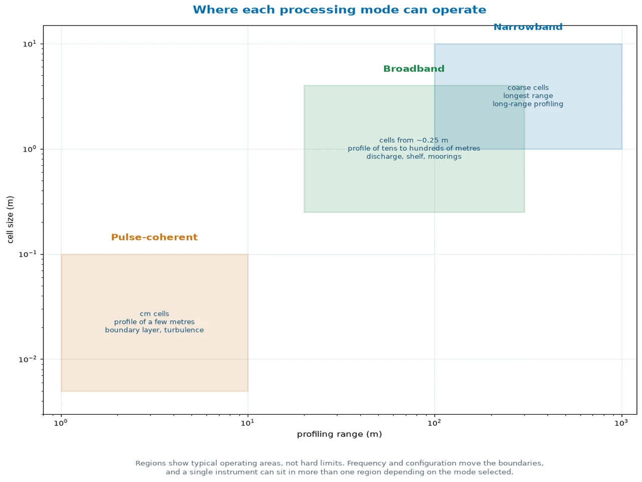
| Typical cell size | Centimetres to a few tens of centimetres | About 0.25 m upward, depending on frequency |
| Typical profile length | A few metres | Tens to hundreds of metres |
| Unambiguous velocity | Hard limit set by lag and wavelength | Wide; not the binding constraint in normal use |
| Short-term precision | Very high | High |
| Averaging requirement | Short range, weak echo — averaging matters | Robust with standard averaging |
| Behaviour in fast flow | Can alias and produce plausible wrong data | Designed for metre-per-second flows |
| Best fit | Boundary layer, turbulence, near-bed sediment flux | Discharge, shelf and slope profiles, moorings, vessel surveys |
The figures are typical rather than universal. The same instrument at the same frequency can sit anywhere in these ranges depending on configuration, and the limits should be checked against the planned cell size, profile length and maximum velocity.
Frequency shifts the whole envelope as well. A 600 kHz instrument reaches about 70 m, a 300 kHz instrument about 160 m and a 75 kHz instrument several hundred metres, with the same relationship between cell size and range applying inside each band. Choosing the processing mode and choosing the frequency are therefore decisions that interact: a mode that gives centimetre cells at 600 kHz will not deliver the same resolution at 75 kHz, where the wavelength is four times longer.
4. Resolution: what cells you actually get
Cell size is set by the transmit pulse length, regardless of mode: a 1 cm cell requires a pulse of roughly 13 microseconds in seawater. Pulse-coherent configurations exist to make pulses that short useful, which is why published near-bed studies report cells of 0.01 to 0.02 m and, in one sediment flux application, roughly 0.7 cm.
Broadband processing uses coded pulses that are longer in duration, so practical cells typically start at about 0.25 m and increase with profile length. That is a large difference in resolution, but it is not a defect: a 0.5 m cell across a 30 m water column produces a useful profile of the whole column, which is the information most discharge and monitoring programmes need.
5. Velocity range and ambiguity
The velocity difference between the modes is the one that catches people out. A pulse-coherent configuration with a 10 ms lag at 1 MHz has an unambiguous velocity of about 3.8 cm/s. That is well matched to a quiescent boundary layer and hopeless in a river flowing at 1 m/s.
Broadband processing is not free of ambiguity effects, but the coded transmission pattern and correlation processing are designed so the usable velocity range matches the environments the instruments are deployed in — estuarine and river flows, tidal channels, coastal and shelf currents. In practice this is why discharge measurement uses broadband or narrowband modes.
ISO 24578 is explicit that if the coherent processing range or maximum velocity limit is exceeded, the measurement data can lose validity. The check is simple and should happen before deployment: compare the site's expected maximum velocity with the mode's limit at the chosen lag, and confirm the profile length required is inside the mode's range.
The underlying reason the two constraints move together is that the product of maximum range and unambiguous velocity is fixed for a given frequency, approximately c²/(8f). Improving one always costs the other. Broadband processing relaxes the coupling rather than removing it, which is why it can cover both a useful profile length and the velocities found in real channels — but not with centimetre cells. The derivation and worked examples are set out in the companion article on the range-velocity trade-off.
6. Which mode for which measurement
| Measurement objective | Typical conditions | Recommended mode |
|---|---|---|
| River or canal discharge measurement | Full depth, 0.2–3 m/s | Broadband |
| Estuarine and tidal channel profiles | Tens of metres, reversing flow | Broadband |
| Shelf, slope and open-ocean moorings | 50–500 m profile | Broadband, or narrowband for the longest ranges |
| Vessel-mounted transect surveys | Moving platform, wide sections | Broadband |
| Near-bed velocity profile and bed shear | Lowest 1–3 m, slow to moderate flow | Pulse-coherent |
| Suspended sediment flux near the bed | Centimetre-scale layering | Pulse-coherent |
| Bottom boundary layer turbulence | Low flow, high sampling rate | Pulse-coherent |
| Fine-scale shear and internal wave structure | Short range, stratified water | Pulse-coherent |
| Very long range with coarse cells acceptable | Hundreds of metres | Narrowband |
Two related articles go into the application detail: sediment monitoring with ADCPs for the near-bed case, and river discharge measurement for the broadband case.
Programmes with mixed objectives are common. A port monitoring project, for example, may need a broad current profile through the water column for navigation and dredging decisions, plus a resolved near-bed layer for siltation studies. That is not a reason to compromise on one mode; it is a reason to define the two requirements separately and match each to its own configuration.
7. Can one instrument do both?
Often, yes — but not at the same time in the same profile. Profiling ADCPs commonly support several processing modes, and switching modes is a configuration change that redraws the whole envelope: cell size, profile length, velocity ceiling and averaging requirements all move together. That makes mode switching practical between deployments, and impractical mid-profile.
Where a programme needs both fine near-bed structure and a full-column profile, the usual answers are:
- Two instruments, one frame. A broadband profiler covers the water column while a pulse-coherent configuration resolves the lowest metre or two, with both records sharing a time base.
- Dual-frequency deployment. Different frequencies give different combinations of range, resolution and ambiguity, and the records are complementary. The trade-offs are covered in our article on dual-frequency ADCP deployments.
- Sequential deployments. Use broadband for the routine record and add a dedicated near-bed campaign when the boundary layer question arises.
In all three cases the planning work is the same: define the layer to be resolved, the maximum flow speed and the profile length, then allocate each requirement to the mode that can meet it.
For long unattended deployments, mode choice also affects the power and data budget. Finer cells over a short range can mean more cells to store and more processing per profile, while a long broadband profile with standard averaging is comparatively predictable. Where telemetry is involved, the transmitted configuration should be the one that answers the monitoring question rather than the one with the most detail available.
8. Configuration checklist
| Setting | Why it matters | Check |
|---|---|---|
| Acoustic frequency | Sets wavelength (velocity limit), attenuation and attainable range | Matched to depth, resolution and expected flow; see the frequency selection guide |
| Cell size and number of cells | Sets resolution and how much of the profile is covered | Cell size small enough for the thinnest layer of interest; see ADCP configuration |
| Pulse separation (coherent) or coding (broadband) | Defines range and velocity envelope | Both the profile length and the maximum velocity inside the envelope |
| Averaging and sampling rate | Controls variance and temporal resolution | Enough pings per average for the noise level; burst mode where waves are involved |
| Blanking and boundary standoff | Side-lobe and near-field effects limit the first and last usable cells | Lowest usable cell documented; not assumed to reach the bed |
| Signal-to-noise ratio | Depends on scatterers in the water | Deployment plan accounts for clear or sediment-laden water conditions |
9. Common mistakes
9.1 Choosing pulse-coherent because "it is more precise"
Precision within a short range and a low velocity ceiling is not precision for a whole river section. If the site exceeds the ambiguity limit, the record is not merely noisier; it is wrong in a way that looks plausible.
9.2 Assuming broadband's cell size equals pulse-coherent resolution
A 0.25 m broadband cell over a 30 m column is a good profile, but it will not resolve a 20 cm boundary layer. Matching mode to layer thickness is the first decision, not the last.
9.3 Ignoring the averaging trade-off
Higher sampling rates reduce the number of pings available to average, so individual estimates can become noisier even though the data arrive faster. In wave-dominated conditions the sampling scheme should follow the process timescale.
9.4 Forgetting boundary effects
Side lobes can return energy from the bed before the main lobe reaches it, so there is a standoff below which data are unreliable. This is relevant whenever near-bed or structure-mounted measurements are planned — including outfall and port monitoring, as described in our articles on outfall monitoring and port and harbour monitoring.
9.5 Treating mode switching as a free option
Every mode change alters range, resolution, velocity limits and averaging, so a configuration that worked in one mode cannot simply be toggled into another without re-checking the deployment plan.
9.6 Reusing a configuration without checking the site
A profile that worked in a sheltered harbour may exceed the velocity limit in a tidal channel with stronger springs, and a cell size that resolved the near-bed layer at one site may be too coarse where the bed is smoother. Site conditions change between deployments, and the mode check should be repeated for each one.
9.7 Comparing cell counts as if they were equivalent
Two profiles with the same number of cells but different cell sizes describe very different water columns. Comparing instruments by cell count rather than by the layer each configuration resolves is a common source of confusion in specifications and tenders.
10. What the standards say
ISO 24578 describes the three processing families, notes the low short-term uncertainty that coherent processing can achieve, and warns that exceeding the coherent range or maximum velocity limits can invalidate the data. Where a derived quantity such as a transport estimate has to be reported formally, the uncertainty framework in ISO 25377 (HUG) applies to the combination of contributing terms, and the parameter selection guidance in our article on key ADCP selection parameters covers the rest of the specification.
11. Frequently asked questions
What is the difference between broadband and pulse-coherent ADCP?
Both use pulse pairs and phase information. Pulse-coherent waits for the first echo before sending the second pulse, tying range to the pulse separation. Broadband transmits coded pulses that can overlap in the water and recovers range and velocity by correlation, allowing a longer profile over a wider velocity range at coarser resolution.
Which mode is more accurate?
Pulse-coherent gives the lowest short-term velocity uncertainty and the finest cells, within a short profile and below its velocity limit. Broadband gives high precision across a long profile. Delivered accuracy depends on whether the mode suits the site.
Which mode should I use for river discharge measurement?
Broadband or pulse-incoherent. Discharge needs a full-depth profile and commonly involves 0.2–3 m/s flow, which exceeds the unambiguous velocity of a practical pulse-coherent configuration.
What cell size does each mode provide?
Pulse-coherent configurations deliver cells from centimetres to a few tens of centimetres over a few metres of profile; published studies report 0.01–0.02 m, and one near-bed study used roughly 0.7 cm. Broadband instruments typically give cells from about 0.25 m upward over tens to hundreds of metres.
Why does pulse-coherent have a velocity limit?
Phase is only measurable within one cycle, so the velocity producing a half-cycle phase shift sets the ceiling. Flows above it appear as plausible but incorrect values, so the site's maximum velocity has to be checked before deployment.
Can one ADCP use both modes?
Many profiling instruments support several modes, but switching changes cell size, range, velocity limits and averaging, so it is practical between deployments rather than mid-profile. Where both fine near-bed detail and a full-column profile are needed, two instruments or a dual-frequency deployment are the usual solutions.
Is narrowband processing still relevant?
Yes, for long-range profiles and difficult conditions where a coarse cell is acceptable. Narrowband transmits one long pulse and estimates the Doppler shift from the echo spectrum, giving long range and robustness with lower spatial resolution.
How do I decide between the two modes?
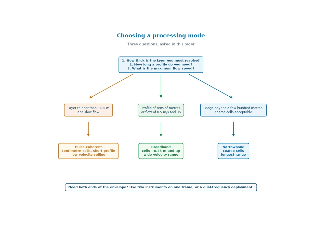
Start with the layer to be resolved and the maximum expected flow speed. A target layer thinner than about half a metre in slow flow points to pulse-coherent. A profile spanning tens of metres or flow reaching metres per second points to broadband.
12. Conclusion
The choice between broadband and pulse-coherent processing is not a choice between a good mode and a lesser one. It is a choice about which part of the measurement envelope matters: centimetre cells within a few metres and a low velocity ceiling, or cells of a fraction of a metre across tens to hundreds of metres of water column with a velocity range that matches real rivers and coastal seas.
Deciding on the layer thickness, the profile length and the maximum flow speed — in that order — resolves the question in most projects. Where both ends of the envelope are required, the answer is usually a combined deployment rather than a compromise configuration.
Published by Oceantek engineering team.Lasted update:September 24,2026.