Executive summary
Ocean upwelling is a transport process, not a temperature event. Water that arrives at the surface from depth carries nutrients, modifies oxygen and carbon distributions, and shapes the productivity of some of the most important fisheries in the world. Temperature and salinity records show that something changed; they do not show how the water moved. An acoustic Doppler current profiler supplies that missing hydrodynamic view, resolving current speed and direction through the water column. This article explains what ADCP observations can and cannot resolve in an upwelling study, how the instruments are deployed, and how to match the specification to the site.
Contents
- Why measure ocean upwelling?
- What is ocean upwelling?
- What an ADCP measures in an upwelling study
- Can an ADCP really measure upwelling?
- How ADCP data characterise the upwelling process
- Deployment methods for upwelling research
- ADCP and CTD: why velocity alone is not enough
- Designing an upwelling observation programme
- Choosing the frequency for upwelling studies
- How to choose an ADCP for upwelling research
- Challenges and limitations
- ADCP compared with other current measurements
- Where upwelling observation is heading
- Frequently asked questions
Why measure ocean upwelling?
Upwelling regions cover a small fraction of the ocean surface and produce a disproportionate share of its fish catch. The reason is nutrient supply: water that has been below the euphotic zone for months or years returns to the surface carrying nitrate, phosphate and silicate, and phytoplankton respond within days. The consequences run through the ecosystem into fisheries, oxygen distribution and the ocean carbon cycle.
Measurement programmes are usually driven by one of four needs: understanding the physical mechanism of upwelling at a particular site, quantifying nutrient or carbon flux, supporting fisheries and ecosystem assessments, or validating a circulation model. All four need the same first-order information, which is how the water moves. Temperature and salinity tell you that subsurface water has reached the surface. They do not tell you the pathway it took, the current structure that carried it, or the shear and mixing along the way.
This is where ADCP measurements become valuable. A current profiler records the velocity field through the water column at the same location and at the same time as the property measurements, which is what allows the physical mechanism and the observed water-mass change to be connected.
What is ocean upwelling?
Definition
Upwelling is the upward movement of deeper water towards the surface. In most cases the water arrives cold and nutrient-rich relative to the surface layer it replaces, so the surface expression of upwelling is a temperature anomaly. The transport, however, is the physical event.
What causes upwelling
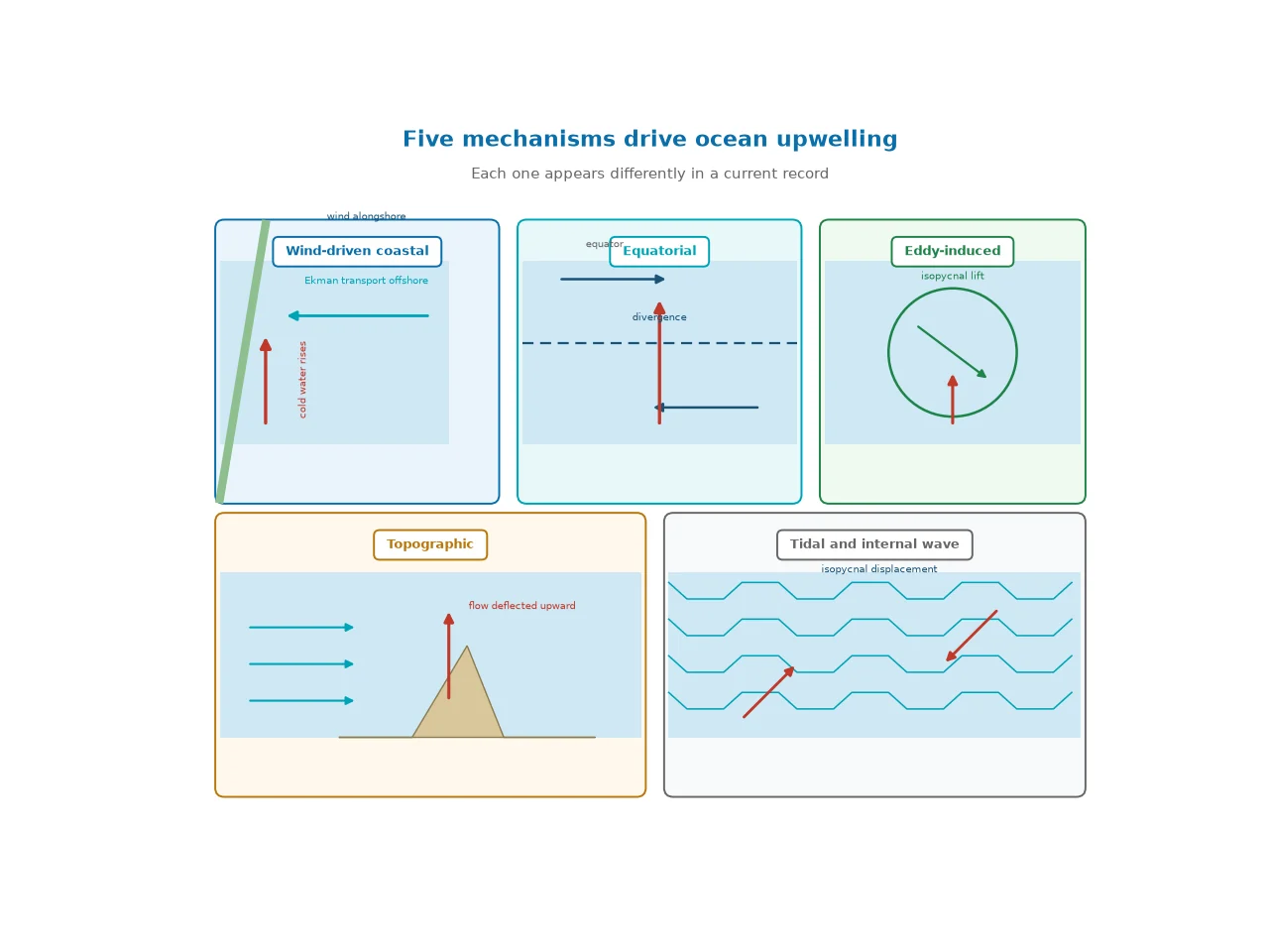
- Wind-driven coastal upwelling. Alongshore wind drives surface water offshore through Ekman transport, and deeper water rises to replace it. The cross-shore transport per unit length of coast follows M = τ / (ρ f), where τ is wind stress, ρ water density and f the Coriolis parameter. This is the classic eastern-boundary upwelling system.
- Equatorial upwelling. The change in sign of the Coriolis parameter across the equator produces divergence in the surface flow, and water upwells along the equator, most strongly in the eastern Pacific and Atlantic.
- Eddy-induced upwelling. Mesoscale eddies displace isopycnals, so water can be lifted hundreds of metres without any coastal boundary. The vertical velocities are small and episodic, which makes them hard to capture.
- Topographic upwelling. Flow interacting with seamounts, ridges, shelf edges and canyon walls is deflected upward. The signal depends on the incident current and the shape of the topography.
- Tidal and internal-wave transport. Internal tides and nonlinear internal waves move water vertically over short time scales, often with strong shear in the upper water column.
Why upwelling is difficult to observe
Upwelling velocity is small. Horizontal currents at an upwelling site can reach 0.5 to 1 m/s; the vertical velocity that actually lifts water to the surface is typically three to four orders of magnitude smaller, in the range of millimetres to a few centimetres per second. A measurement programme therefore has to resolve a weak vertical signal against a large horizontal flow, and it has to do so while the event evolves over days to weeks.
Property measurements alone cannot close that gap. A CTD cast that shows cold, salty water at the surface records the result of transport, not the transport itself. To describe the mechanism, the programme needs the velocity field as well, which is what an ADCP contributes.
What an ADCP measures in an upwelling study
Current velocity profiles
An ADCP transmits acoustic pulses along beams and derives velocity from the Doppler shift of echoes returned by scatterers in the water. The measurement is divided into depth cells, so the instrument returns a profile rather than a single value: current speed and direction in each cell, from the transducer to the limit of its range. In an upwelling study, that profile is what allows the horizontal flow to be separated from the vertical structure it produces.
Horizontal current structure
On a coastal upwelling margin the horizontal structure has a consistent geometry: an alongshore current that is usually equatorward, a cross-shore component that reverses during the upwelling and relaxation phases, and a vertical structure in which surface and subsurface flow can differ in both speed and direction. A moored ADCP resolves that structure continuously, and a shipboard ADCP maps it across the shelf.
Vertical velocity and vertical transport
ADCPs measure a vertical velocity component as part of the three-dimensional solution, and it is tempting to present that number as the upwelling rate. That would overstate what the measurement supports. Several factors limit the interpretation:
- Magnitude. Vertical velocities in the open ocean are commonly a few millimetres per second, close to the resolution of the instrument.
- Sensitivity to geometry. A small instrument tilt changes the projection of the horizontal flow onto the vertical axis, and tilt is rarely constant on a mooring.
- Noise and averaging. Vertical estimates improve with averaging over time and space, but averaging also smooths the short-lived events that matter.
- Sample volume. The vertical beam samples a different volume from the slanted beams, so the comparison is not always straightforward in strongly sheared flow.
In practice, vertical transport is inferred from a combination of vertical velocity estimates, horizontal divergence and convergence in the measured profile, vertical shear, and mass continuity, with temperature and salinity data used to check that the inferred transport is consistent with the observed water-mass change. This is the standard approach in upwelling analysis, and it is the reason an ADCP is usually deployed alongside a CTD rather than on its own.
Can an ADCP really measure upwelling?
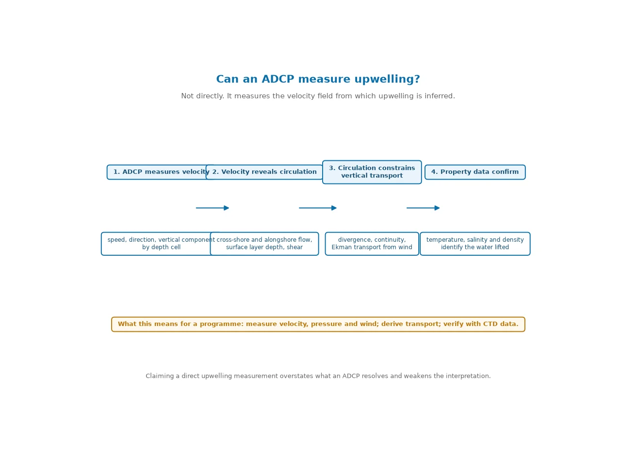
The honest answer is that an ADCP does not measure upwelling directly. It measures the velocity field from which upwelling is inferred, and the strength of the inference depends on how the data are used. The chain has four links:
- ADCP measures velocity. Profiles of horizontal velocity, vertical velocity and, on many instruments, echo intensity, in depth cells through the water column.
- Velocity reveals circulation. The measured structure identifies cross-shore and alongshore flow, the depth of the surface layer, and the shear between water masses.
- Circulation constrains vertical transport. Horizontal divergence, continuity and the observed shear set limits on how much water must be moving vertically to balance the flow. Wind stress and Ekman theory provide an independent estimate where wind data are available.
- Property data confirm the result. Temperature, salinity and density from a CTD show whether the water being lifted is consistent with the transport inferred from the current field.
Presenting the chain this way matters for two reasons. It avoids the technical error of claiming a direct upwelling measurement, and it shows where each instrument contributes, which is the information a reviewer or referee will look for. If a project needs a formal uncertainty statement for a derived transport estimate, the framework in ISO 25377 (HUG) applies to the combination of terms.
How ADCP data characterise the upwelling process
An upwelling event has a recognisable sequence in a current record, and the sequence is often as informative as the peak values.
Detecting changes in current structure
- Before the event: relatively stable alongshore flow with a shallow surface layer and weak cross-shore transport.
- During the event: stronger cross-shore circulation, increased vertical shear, and a surface layer that deepens or reorganises as colder water arrives.
- After the event: relaxation of the cross-shore flow, often followed by a period of downwelling or alongshore advection that redistributes the new water.
Measuring current shear
Shear is the velocity gradient with depth, and it carries information that a single current speed cannot. Surface and subsurface currents at an upwelling site often differ in direction as well as speed, and a strong gradient marks the boundary between water masses. Shear also controls mixing, so it links the physical forcing to the biological response: the rate at which nutrients are mixed into the euphotic zone depends on the stability and shear of the upper water column, not only on how much water is upwelled.
Identifying circulation patterns
With a time series of profiles, four patterns can be separated: onshore and offshore flow at different depths, the alongshore jet that dominates many upwelling margins, vertical circulation connecting them, and the compensating flows that close the mass balance. Combining a moored record with a shipboard section provides both the time evolution at a point and the spatial extent of the pattern.
Deployment methods for upwelling research
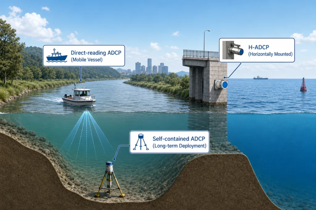
Bottom-mounted ADCP
The instrument sits on a seabed frame and profiles upward. The position is stable, no surface expression is required, and continuous records of several months are routine with a self-contained instrument. This configuration suits coastal upwelling stations on the shelf, where the water column is within the profiling range. Mooring and frame design is covered in more detail in our guide to mounting solutions for buoys, tripods and fixed platforms.
Moored ADCP
Mounted on a subsurface or surface mooring line, the instrument can sit at the depth where the signal of interest is strongest rather than near the bed, and it can be placed in deep water beyond the range of a seabed installation. Moorings are the standard tool for seasonal and multi-year time series, including the equatorial arrays that underpin much of what is known about equatorial upwelling.
On a mooring that sits deeper than the shelf, the profiling range becomes the limiting specification, because the instrument still has to see the surface layer where the upwelling signature appears. A 300 kHz profiler covers about 160 m; the 150 kHz Ocean-ADCP-150-PA4 extends that to 250–400 m in a housing rated to 6,000 m, which is the range that matters for slope and mid-depth upwelling moorings.
Shipboard ADCP
Hull-mounted or over-the-side instruments measure while the vessel moves, producing sections of current structure across a shelf or a frontal region in days. The trade-off is the opposite of a mooring: spatial coverage is excellent, temporal coverage depends on how often the section is repeated. For upwelling work, the practical combination is a mooring for the time series and repeated shipboard transects for the spatial pattern, with the two reconciled through overlapping measurement periods.
ADCP and CTD: why velocity alone is not enough
Every instrument in an upwelling programme answers a different question. Treating the ADCP as a complete solution leads to a weak interpretation, because velocity alone cannot identify the water being transported.
| Instrument | What it measures | What it contributes to an upwelling study |
|---|---|---|
| ADCP | Current speed and direction by depth cell; vertical velocity component; echo intensity | How the water moves: circulation, shear, divergence and transport constraints |
| CTD | Temperature, salinity, density | Which water is moving, and whether it is consistent with the inferred transport |
| Temperature loggers | Time series of temperature at fixed depths | Timing of the event and the vertical extent of the cold-water intrusion |
| Wind sensors or reanalysis | Wind speed and direction | Forcing: upwelling-favourable wind stress and Ekman transport estimates |
| Turbidity sensors | Suspended material | Near-bed transport and resuspension during active periods |
| Chlorophyll or oxygen sensors | Biological and chemical response | Whether the physical event produced the expected ecosystem response |
Designing an upwelling observation programme
The following structure reflects how an upwelling observation programme is normally assembled. It is a design pattern rather than a published data set: the numbers depend on the site, and the interpretation is what the programme has to produce.
Study setting
A seasonal upwelling margin with a shelf within the profiling range of a moored or seabed instrument, and a wind record that shows distinct upwelling-favourable and relaxation phases.
Instrument suite
- ADCP on a seabed frame or subsurface mooring, configured with cell sizes matched to the depth of the surface layer;
- CTD profiles at the mooring site and along the shipboard section;
- temperature loggers at two or three depths for event timing;
- wind observations or reanalysis products covering the deployment period;
- optional turbidity and chlorophyll sensors for transport and response.
Observation period
Long enough to contain several upwelling cycles and at least one full relaxation, which in most seasonal systems means weeks to months rather than days.
Data interpretation
The interpretation follows the sequence that the instruments are designed to resolve: upwelling-favourable wind stress, change in the surface current, modification of the vertical current structure and shear, upward transport of colder and denser water, and detection of the event in the property record. Presenting the chain in that order makes the physical argument explicit and shows which measurement supports each step.
Choosing the frequency for upwelling studies
Frequency sets the trade-off between profiling range and vertical resolution, and the choice follows the water depth and the structure the programme needs to resolve rather than any general rule that a higher frequency is better. Four bands cover most upwelling deployments: 600 kHz for nearshore work, 300 kHz on the shelf, 150 kHz where a deep mooring still has to reach the surface layer, and 75 kHz for the longest profiles.
| Site and task | Typical depth | Priority | Suitable configuration |
|---|---|---|---|
| Nearshore upwelling station, upper water column structure | <50 m | Fine vertical cells, compact mooring or frame | 600 kHz profiling ADCP; compact phased-array 600 kHz where space is tight |
| Shelf mooring, coastal to mid-shelf section | 50–150 m | Range with usable resolution near the surface | 300 kHz profiling ADCP |
| Slope and mid-depth mooring | 150–400 m profile | Reaching the surface layer from a deep mooring | 150 kHz Ocean-ADCP-150-PA4, 250–400 m profile, rated to 6,000 m |
| Offshore and deep-basin deployments | >400 m profile | Maximum profiling range | 75 kHz phased-array ADCP, 650 m range |
| Long-term unattended station | Site dependent | Internal recording, battery endurance | Self-contained ADCP series |
| Shore or platform fixed station | Shallow coastal | Continuous coverage from a fixed point | Horizontal ADCP for horizontal profiling from a structure |
Frequency choice is covered in more depth, including the full comparison across the 75, 300 and 600 kHz bands, in our guide to ADCP frequency selection.
How to choose an ADCP for upwelling research
Required profiling range
Start from the water depth and the part of the column that must be resolved. On a 60 m shelf, a 600 kHz instrument covers the range with fine cells. On a 150 m slope mooring, a 300 kHz instrument is more suitable. Where a mooring sits at 300 m or deeper and still has to resolve the surface layer, the 150 kHz Ocean-ADCP-150-PA4 provides 250–400 m of profile; the 75 kHz band is reserved for the deepest deployments. Where the surface layer itself is the target and the instrument is on the seabed, check the range against the deepest expected mixed layer rather than the mean depth.
Vertical resolution
Cell size, cell count and profiling range are linked. Fine cells near the surface layer boundary are usually more valuable than uniform cells through the whole column, and many instruments allow cell size to be configured for exactly that reason. The trade-off is documented in our guide to ADCP configuration.
Measurement accuracy
Velocity accuracy matters, but so do bias and signal-to-noise ratio, because upwelling analysis depends on small differences between large numbers. Specifying accuracy without considering how the data will be averaged and processed is a common omission; the general parameters are set out in our article on the key parameters for selecting an ADCP.
Deployment method
Frame, mooring or vessel mounting determines what the instrument can observe. A frame gives an uninterrupted time series at the bed; a mooring places the measurement at the depth of interest; a vessel gives spatial sections. Projects that need all three should plan overlapping deployment periods so the records can be compared.
Environmental conditions
Salinity, temperature range, pressure rating, biofouling pressure, suspended sediment and wave exposure all affect instrument selection and the maintenance interval. Biofouling is the practical limit on deployment duration in warm coastal water, and it is addressed with antifouling protection and service planning rather than with instrument choice alone.
Data transmission
For a station that has to inform decisions in real time, the data path matters as much as the sensor: serial output at the instrument, then telemetry or a cabled link to shore, with the sampling scheme set so that battery and bandwidth are used for the periods that matter. Where real-time delivery is not required, an internally recording self-contained instrument simplifies the deployment.
Challenges and limitations
Weak acoustic backscatter
The measurement depends on scatterers in the water. In clear, low-productivity water, or below the depth where biological scatterers are abundant, the signal weakens and range or resolution has to be traded off.
Surface and bottom boundary effects
No profiler measures the water column completely. There is a blank distance below the transducer, a side-lobe region near the boundary opposite it, and reduced data close to the seabed. In an upwelling study the near-surface data are often the most interesting, so the blanking distance and mounting depth have to be planned rather than accepted.
Vertical velocity measurement limits
Vertical velocity is much smaller than horizontal velocity, which makes the measurement sensitive to instrument tilt, noise, beam geometry and the assumption that the flow is horizontally uniform across the beam spread. Tilt correction helps, but it does not remove the need for careful averaging and for independent checks against property data.
Biofouling
In warm, productive coastal water, growth on the transducer degrades signal quality within weeks. Deployment duration has to be matched to the maintenance plan, and recovery intervals should be planned before the first deployment.
Complex ocean currents
Real flows are not two-dimensional. Internal waves, eddies and topography all superimpose structure on the mean circulation, and the interpretation has to distinguish the mean transport from the variability around it. This is an analysis challenge, but it also determines the sampling scheme: short deployments at high resolution trade against long records that contain the mean signal.
ADCP compared with other current measurements
| Technology | Velocity profile | Spatial coverage | Long-term monitoring | Typical contribution |
|---|---|---|---|---|
| ADCP | Yes, by depth cell | Vertical profile at a point, or a section when vessel-mounted | Yes | Current structure, shear, transport constraints |
| Current meter | Limited, point measurement | Single depth at one location | Yes | Point velocity, redundancy, long records at low cost |
| HF radar | Surface layer only | Large area, tens of kilometres | Yes | Surface current maps for spatial context |
| Drifter | Trajectory, Lagrangian | Path dependent | Limited | Surface transport pathways |
| CTD | Not a velocity measurement | Vertical hydrography | Yes | Water properties, water-mass identification |
The point of the comparison is not that one instrument is best. Different technologies observe different parts of the upwelling system, and the strongest programmes combine them: radar or drifters for surface context, an ADCP for the velocity structure, and a CTD for the properties of the water being moved.
Where upwelling observation is heading
Real-time upwelling monitoring
Telemetered ADCP stations already deliver current profiles to shore as they are measured. For upwelling regions, the practical value is early detection: the current structure often changes before the surface temperature signal is unambiguous, so a real-time velocity record can trigger additional sampling while the event is developing.
Autonomous platforms
Gliders, AUVs and uncrewed surface vessels extend coverage between fixed stations. Their navigation depends on velocity references of the kind a Doppler velocity log provides, and the navigation problem itself is covered in our article on AUV navigation without GPS.
Multi-sensor observatories
Combining ADCP, CTD, oxygen and chlorophyll sensors on one platform produces a record in which the physical forcing and the ecosystem response share a time base. That is the configuration that supports process studies rather than descriptive monitoring.
Model validation and data assimilation
Current profiles are among the few direct measurements available for validating circulation models in upwelling regions, and they are increasingly assimilated rather than used only for post-hoc comparison. A well-documented mooring record with known uncertainty is more valuable in that context than a larger data set without metadata.
Frequently asked questions
What is an ADCP used for in oceanography?
It measures current velocity through the water column. In oceanography that supports current structure studies, transport estimates, mooring and observatory time series, shipboard sections, and velocity references for circulation models and for other instruments.
Can an ADCP measure ocean upwelling?
Not directly. An ADCP measures water velocity and current structure, which are used to characterise the circulation and vertical transport associated with upwelling. Interpreting an upwelling event normally combines ADCP velocity data with temperature, salinity and wind measurements.
Can ADCP measure vertical currents?
ADCPs provide a vertical velocity component, but ocean vertical velocities are typically millimetres to centimetres per second, close to the noise floor of the measurement, and sensitive to tilt and beam geometry. Vertical transport is therefore normally inferred from a combination of vertical velocity, horizontal divergence, shear and continuity, checked against property data.
What ADCP frequency is best for ocean upwelling studies?
It depends on water depth and required vertical resolution. 600 kHz suits nearshore and shelf deployments with fine cells; 300 kHz profiles to about 160 m; a 150 kHz phased-array instrument covers 250–400 m for slope and mid-depth moorings; 75 kHz reaches several hundred metres in deep water at coarser resolution.
Can an ADCP be deployed on the seafloor?
Yes. Seabed frames are common for coastal upwelling monitoring because the position is stable, the instrument can record for months, and an upward-looking profile covers the water column from the bed towards the surface.
What is the difference between a moored ADCP and a shipboard ADCP?
A moored ADCP produces a time series at one location. A shipboard ADCP produces spatial sections while the vessel moves. Upwelling programmes often use both: moorings for event evolution and shipboard surveys for spatial extent.
Can ADCP data be combined with CTD measurements?
Yes, and it is standard practice. The ADCP records how the water moves; the CTD records temperature, salinity and density structure, which identifies the water mass being transported.
How deep can an ocean ADCP measure?
Profiling range depends on frequency and site conditions: roughly 70 m at 600 kHz, around 160 m at 300 kHz, 250–400 m at 150 kHz, and several hundred metres at 75 kHz. The housing pressure rating is a separate specification and reaches 6,000 m.
This article describes measurement methods for general information. Instrument specifications and configurations should be confirmed for your site and deployment method before a programme is designed.