Executive summary
An ADCP is not part of the desalination process — it is the instrument that tells you how the sea is moving around your intake and outfall. This guide covers the six ways ADCPs are used in seawater desalination projects, which Oceantek model fits each job, and — just as importantly — what an ADCP cannot do, so monitoring programmes are designed with the right instrument stack.
Contents
- Why desalination projects need current data
- Intake siting and entrainment risk
- Outfall design: baseline current data
- Brine plume monitoring and mixing-zone compliance
- Long-term unattended monitoring
- Construction and marine works
- Real-time telemetry and adaptive sampling
- Model selection matrix
- What ADCPs cannot do in desalination
- Deployment checklist
- Equipment in practice
- FAQ
1. Why desalination projects need current data
Seawater reverse osmosis (SWRO) plants take in large volumes of seawater and return a concentrated brine. Both ends of that exchange depend on the sea itself: the intake has to draw water without capturing the wrong things, and the outfall has to release brine into a receiving environment that mixes and disperses it acceptably.
Brine typically leaves the plant at roughly twice the salinity of the source seawater and, because it is denser, it behaves differently from a normal effluent: instead of simply floating away, it tends to sink and spread along the seabed, unless a diffuser and ambient mixing lift it into the water column. Where it goes, how fast it dilutes, and whether it stays within a permitted mixing zone are all questions about water movement.
That is where current measurement enters the project:
- Intake design needs the local current field to assess entrainment and impingement risk, sediment transport and intake siting;
- Outfall design needs measured currents — often resolved by depth — as input to near-field and far-field plume models;
- Compliance monitoring needs a record of ambient currents to interpret plume behaviour and demonstrate that dilution is being achieved;
- Operations benefit from real-time current data for sampling, maintenance windows and anomaly detection.
2. Intake siting and entrainment risk
An intake structure pulls seawater — and whatever is travelling in it. The environmental concern is twofold: entrainment (small organisms, eggs and larvae drawn into the plant) and impingement (larger organisms trapped against screens). Both are strongly influenced by the local current field, which determines how larvae and sediment are transported towards the intake and how quickly they are replenished from elsewhere.
ADCP measurements support this work in two ways:
- Long-term seabed monitoring captures tidal cycles, spring–neap variation and seasonal change in current speed and direction near the proposed intake — the variability that determines exposure over time;
- Vessel-mounted surveys map the spatial structure of the flow, including the depth-varying currents and frontal features that a fixed instrument cannot see.
Typical instrumentation: Ocean ADCP 300-FA4 for shelf and mid-depth sites, Ocean ADCP 600-FA4 for shallow nearshore positions, and a HADCP-600 when a fixed station is needed to monitor the intake approach continuously. For the coastal measurement context, see our article on ADCPs for coastal studies.
3. Outfall design: baseline current data
Outfall design is a modelling exercise built on measured data. Plume models — whether near-field models for the diffuser or far-field models for regional dispersion — need to know the ambient currents the plume will be released into:
- current speed and direction through the water column, because stratification controls where the brine ends up;
- tidal phase, because dilution varies dramatically between ebb, flood and slack water;
- seasonal extremes, because the design case is usually the worst-case condition, not the average;
- long-term statistics, to characterise how often the mixing zone is likely to be exceeded.
Because of this, baseline deployments typically run for at least one full seasonal cycle, and stratified sites often need instruments at more than one depth. Self-contained ADCPs that record internally with battery power are the practical choice for these unattended campaigns, and the resulting records feed directly into the plume modelling work.
Typical instrumentation: self-contained ADCPs in the 300 kHz and 600 kHz classes for shelf and coastal sites, and the 75 kHz 75-PA4 where the outfall sits in deep water and long profiling range is needed.
4. Brine plume monitoring and mixing-zone compliance
Once the plant is operating, monitoring shifts to verification: is the brine diluting as predicted, and does it stay inside the permitted mixing zone? This is the best-established ADCP application in desalination, and it is usually a two-part programme:
- Vessel-mounted surveys cross the plume from the diffuser towards the edge of the mixing zone, mapping current structure at the same time as the CTD records salinity and density — so the flow field and the plume can be interpreted together;
- Fixed-station monitoring provides a continuous ambient-current record against which individual surveys and model predictions can be compared.
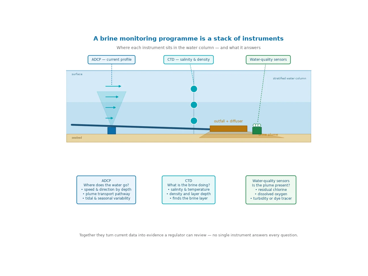
For the physics of dilution — near-field versus far-field behaviour, stratification and dense brine plumes — see our dedicated guide on outfall monitoring with ADCPs.
5. Long-term unattended monitoring
Environmental programmes in this sector are rarely short. Baseline studies run for seasons, and operational compliance may run for the life of the plant, so instruments have to survive and record without an operator present.
- Self-contained ADCPs (battery and internal memory) are deployed on seabed frames and recovered periodically for data download;
- Deployment duration is set by battery capacity, sampling scheme and memory — a trade-off between resolution and how long the instrument can stay down;
- Biofouling and sediment are the practical enemies: antifouling protection, careful mounting height and servicing intervals keep the data usable.
Typical instrumentation: the self-contained ADCP series in 75, 300 and 600 kHz versions, matched to site depth.
6. Construction and marine works
Before a plant operates, it has to be built: intake and outfall pipelines are laid, diffuser structures installed, channels dredged and rock placed. Current data supports this phase in three ways:
- Work windows — knowing when currents are within the limits of divers, ROVs and installation vessels;
- Dredging and sediment management — tracking how suspended material moves away from the works;
- Post-lay inspection — ROV and AUV surveys along the pipeline, where a DVL provides the underwater navigation that keeps survey data positioned correctly.
Typical instrumentation: 600 kHz and 300 kHz profiling ADCPs for vessel and seabed deployment, and the DVL series for ROV/AUV navigation.
7. Real-time telemetry and adaptive sampling
Not every measurement needs to be processed months later. A fixed station can stream current data continuously, which changes what a monitoring programme is able to do:
- trigger sampling when currents are carrying the plume towards a sensitive receptor;
- support plant operations and maintenance planning;
- detect anomalies — an unexpected current pattern, or a change in plume behaviour;
- build a continuous compliance record rather than a series of snapshots.
Typical instrumentation: HADCP-600, a horizontal-profiling ADCP designed for fixed-station deployment and telemetry, with a single-point current meter providing a simple, low-cost point measurement or a redundancy channel.
8. Model selection matrix
The choice of instrument is driven by three things: water depth, how the instrument will be deployed, and whether the data is needed in real time or as an archived record.
| Task | Typical site | Deployment | Suggested model |
|---|---|---|---|
| Deep intake / offshore outfall baseline | Deep water (>200 m) | Seabed frame, self-contained | Ocean ADCP 75-PA4 (650 m range) |
| Shelf baseline & seasonal monitoring | Mid-depth (50–200 m) | Seabed frame, self-contained | Ocean ADCP 300-FA4 (160 m range) |
| Nearshore intake / outfall near-field surveys | Shallow (<50 m) | Seabed frame or vessel-mounted | Ocean ADCP 600-FA4 (70 m, high resolution) |
| Compact or space-limited installations | Shallow to mid-depth | Small frame, buoy or structure | Ocean ADCP 600-PA5 (phased array, Ø92 mm) |
| Continuous fixed-station monitoring | Intake or outfall approach | Shore or structure-mounted | HADCP-600 (horizontal, 90 m range) |
| Long-term unattended records | Any depth | Seabed frame, self-contained | Self-contained 75 / 300 / 600 series |
| Simple point current or redundancy | Any depth | Mooring or frame | Single-point current meter |
| ROV / AUV pipeline inspection | Along the outfall route | Vehicle-mounted | DVL series |
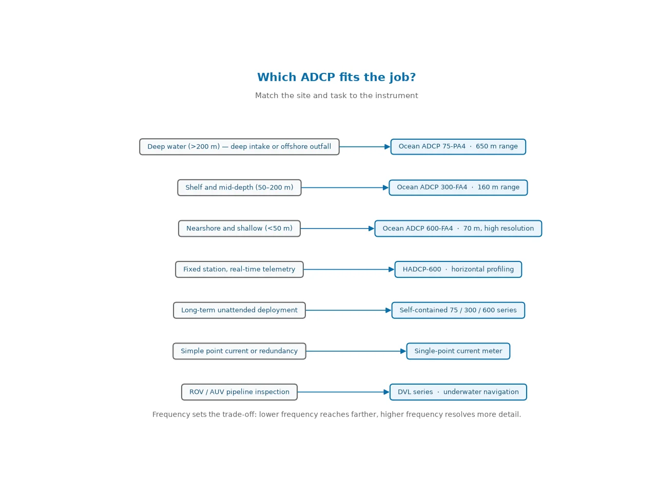
The underlying trade-off is simple: lower frequencies reach farther (75 kHz for deep water and long range), while higher frequencies resolve more detail over shorter distances (600 kHz for nearshore work). Direct-reading versions are used when a cable to a vessel or shore station is practical and data is wanted live; self-contained versions are used when the instrument has to record alone for weeks or months.
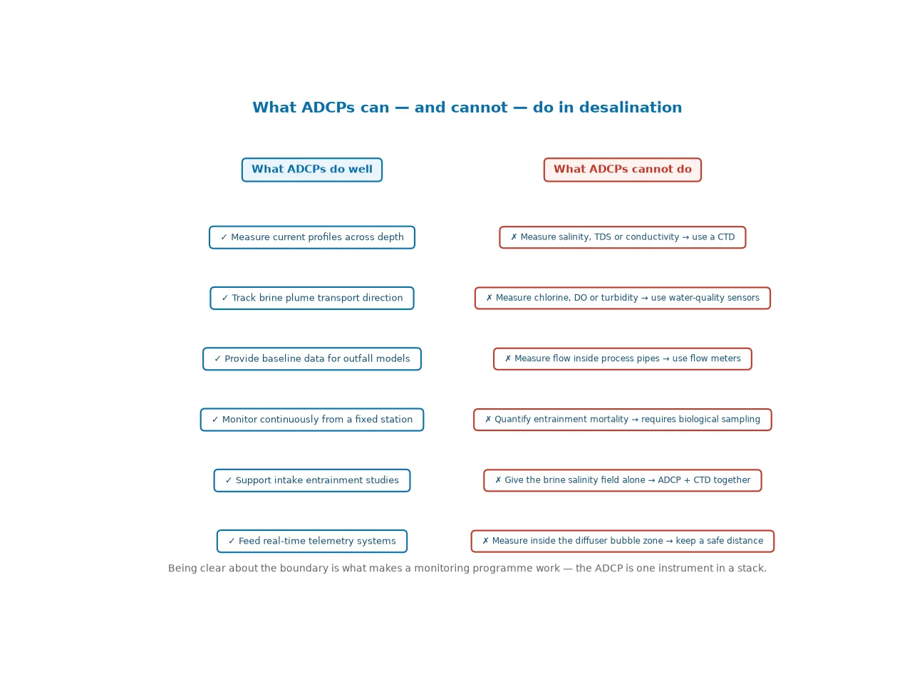
9. What ADCPs cannot do in desalination
This is the section most equipment pages skip — and it is the one that decides whether a monitoring programme actually works.
| An ADCP cannot… | What to use instead |
|---|---|
| Measure salinity, TDS or conductivity | CTD, salinity sensor or multi-parameter probe |
| Report brine concentration or density directly | CTD data plus water samples (density derived from salinity and temperature) |
| Measure residual chlorine, dissolved oxygen or turbidity | Water-quality sensors |
| Measure flow inside process pipes | Electromagnetic or ultrasonic flow meters |
| Produce the brine’s salinity field on its own | ADCP (currents) combined with CTD / towed sensors (salinity) |
| Quantify entrainment mortality | Biological sampling and entrainment assessment methods |
| Measure inside the diffuser’s bubble-rich jet | Keep the instrument outside the jet and measure the ambient field |
| Resolve the very top of the water column or the bed boundary layer | Account for blanking and side-lobe zones; add auxiliary instruments if needed |
10. Deployment checklist
| Phase | Key actions |
|---|---|
| Design / baseline | Define the questions (intake risk, plume modelling, compliance); choose site positions; select frequency for depth and resolution; plan a season-long record; agree the data format the modellers need. |
| Construction | Set work-window thresholds; deploy a vessel-mounted ADCP for real-time support; monitor sediment movement around dredging; use ROV/AUV with DVL for pipeline positioning. |
| Operations | Run fixed-station monitoring with telemetry; conduct periodic vessel and CTD surveys across the plume; maintain and service instruments; archive raw and processed data with QA records. |
| All phases | Antifouling and mounting height; power and data-recovery plan; sound-speed settings for the site; documentation for review and audit. |
11. Equipment in practice
Oceantek’s range covers the deployment types a desalination monitoring programme needs:
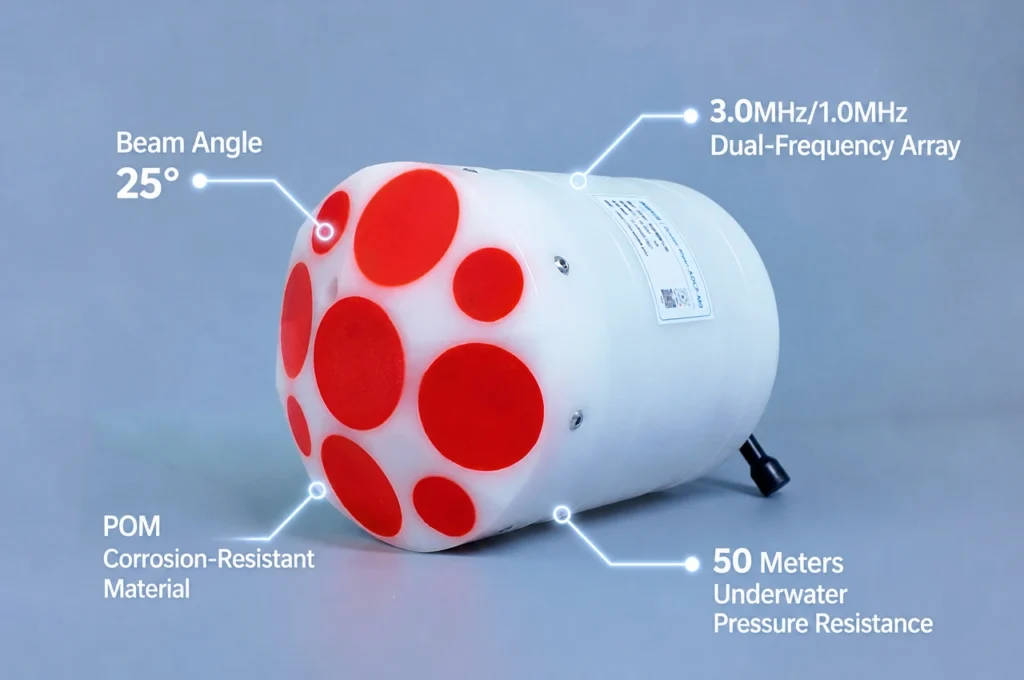
- Ocean ADCP series — 75, 300 and 600 kHz profiling ADCPs in direct-reading and self-contained versions, with depth ratings to 6,000 m for deep outfall and intake work;
- HADCP-600 — horizontal profiling for fixed-station, real-time monitoring of intake and outfall approaches;
- Single-point current meter — a simple point measurement for redundancy or budget-limited programmes;
- DVL series — underwater navigation for the ROV and AUV surveys that inspect outfall pipelines.
One clarification we repeat to every project team: standards describe methods, not instruments. An ADCP is not “ISO certified” for discharge measurement — compliance comes from following the relevant method standard, such as ISO 24578 for moving-boat work, and documenting the result. If your programme needs that framework, our standards overview explains how the pieces fit together.
12. FAQ
Can an ADCP measure salinity?
No. An ADCP measures water velocity, not water chemistry. Salinity, temperature and density come from a CTD or salinity sensor, and parameters such as residual chlorine, dissolved oxygen and turbidity require water-quality instruments. In brine monitoring, the ADCP and CTD work as a pair: the ADCP shows where the water is going, the CTD shows what the brine is doing.
What is an ADCP used for in a desalination plant?
Intake siting and entrainment studies, baseline current data for outfall and plume modelling, brine plume monitoring and mixing-zone compliance, long-term unattended monitoring, construction support, and real-time telemetry at fixed stations.
How do you monitor brine discharge?
Typically with three instruments working together: an ADCP for current profiles and plume transport, a CTD for salinity, temperature and density, and water-quality sensors where the permit requires them. Vessel surveys provide spatial coverage; fixed stations provide continuous records.
Where should ADCPs be deployed at a desalination plant?
Common positions are the seabed near the intake (currents that carry larvae and sediment), the seabed in the outfall mixing zone (ambient currents and plume transport), and a shore or structure-mounted position for continuous real-time monitoring. Vessel-mounted ADCPs cover the space between fixed positions.
How long do ADCP deployments need to run for outfall design?
Long enough to capture the full range of conditions — typically at least one seasonal cycle, including tidal and spring–neap variability, with the record dimensioned for the worst-case design condition.
How many ADCPs does an outfall monitoring programme need?
It depends on site complexity. A simple programme may use one seabed ADCP in the mixing zone plus periodic vessel surveys; stratified or complex sites often need two or more instruments at different depths, plus a fixed station for continuous compliance records.
Can ADCPs be used for intake entrainment studies?
Yes, for the physical side: ADCPs measure the currents that transport larvae, eggs and sediment towards the intake, which underpins entrainment and impingement risk assessment. Biological impact itself is assessed by sampling — the ADCP supplies the flow context.
Do ADCPs work in high-salinity water?
Yes. Acoustic velocity measurement is not affected by salinity the way chemical sensors are, although the speed of sound does vary with salinity and temperature, so sound-speed settings should be configured for the site. Dense brine layers profile normally.
What is the difference between bottom-mounted and vessel-mounted ADCP surveys?
Bottom-mounted and self-contained ADCPs record continuously at one location, capturing tidal and seasonal variability. Vessel-mounted ADCPs survey along a line, mapping spatial structure — for example, crossing the plume from the diffuser to the edge of the mixing zone.
Can ADCP data feed plume dispersion models?
Yes. Near-field and far-field plume models need measured ambient currents, often resolved by depth, together with tidal phase and seasonal extremes — exactly what a well-designed ADCP deployment provides.
How do you prevent marine growth on long deployments?
Use site-appropriate antifouling protection, keep transducers clear, plan service or recovery intervals, and design the data-recovery method (direct download, removable storage or telemetry) around maintenance access.
What does an ADCP monitoring programme cost to run?
The main drivers are the number of instruments, deployment duration, servicing frequency and whether real-time telemetry is required. A single seasonal baseline deployment costs far less than a year-round, multi-instrument compliance network — so the monitoring plan should follow the permit requirements and the site’s complexity.
This article is provided for general information. Monitoring requirements are set by the applicable permits and regulations for each project, and should be confirmed with the relevant authority and project team.