No single acoustic frequency can optimally profile every river condition. Shallow headwater streams demand high-frequency resolution; deep, turbid channels require low-frequency penetration; and tidal estuaries sit somewhere in between. Dual-frequency ADCP deployments—whether through a single multi-beam instrument or strategically paired devices—solve this fundamental trade-off. This article explains when dual-frequency approaches are necessary, how to execute them correctly, and what the Oceantek River-ADCP-M9 brings to the practice.
The Fundamental Frequency Trade-Off
Every acoustic Doppler current profiler faces the same physical constraint: higher frequencies yield finer spatial resolution but shorter range, while lower frequencies penetrate farther but with coarser resolution. In river environments, this translates into a practical decision matrix:
| Frequency | Max Profiling Range | Typical Cell Size | Best Application | Limitation |
|---|---|---|---|---|
| 3.0 MHz | ~3–5 m | 0.02–0.25 m | Ultra-shallow streams (<1 m); near-boundary resolution | Very limited range; high attenuation in turbid water |
| 1.2 MHz | ~20–25 m | 0.05–0.5 m | Shallow rivers; high-accuracy velocity in low-sediment water | Poor performance in deep or highly turbid channels |
| 600 kHz | ~50–70 m | 0.5–4 m | Medium rivers; good all-around compromise | Undersamples near-bed in deep channels; moderate range in sediment |
| 300 kHz | ~100–150 m | 1–8 m | Deep rivers; high-sediment environments; long-range profiling | Coarse resolution in shallow water; larger blank distance |
This frequency–range–resolution trade-off is why river-type ADCPs are increasingly offered in multi-frequency configurations. The question is no longer “which frequency?” but “which combination of frequencies, and how should they be deployed together?”
When Dual-Frequency Deployment Is Necessary
Dual-frequency ADCP deployment is not a universal requirement. For many monitoring sites with stable, single-regime hydraulics, a well-chosen single frequency is sufficient. Dual-frequency approaches become essential—or at least strongly advisable—under the following conditions:
1. Sites with Extreme Stage Variability
Rivers that swing from baseflow depths of under 0.5 m to flood-stage depths exceeding 10 m cannot be adequately profiled by a single frequency. At low stage, a 300 kHz unit has a blank distance and cell size too coarse to resolve the thin water column; at flood stage, a 1200 kHz unit cannot reach the channel bed. A dual-frequency instrument—or two co-deployed instruments at different frequencies—covers both extremes.
2. Highly Variable Suspended Sediment Concentration (SSC)
Acoustic attenuation scales nonlinearly with both frequency and sediment concentration. During low-SSC baseflow periods, higher frequencies (600–1200 kHz) maintain excellent data quality. During sediment-laden flood pulses—when SSC can exceed 10 kg/m³—higher frequencies lose range rapidly, and lower frequencies (300 kHz) become essential to maintain profiling coverage. Field studies by Moore et al. (2011) demonstrated that 300 kHz and 600 kHz H-ADCPs underestimated velocity during low-flow, low-concentration periods, while 1200 kHz maintained accuracy—confirming that no single frequency is optimal across all sediment regimes.
3. Tidal Rivers and Backwater-Affected Reaches
In tidally influenced or backwater-affected reaches, flow direction reverses and velocity profiles become non-logarithmic and highly variable across the vertical. Multi-frequency deployments are particularly valuable here because the index-velocity method depends on capturing representative velocities—and a profile measured at the wrong frequency may miss critical near-bed or near-surface flow features. Recent research at Zhicheng Station (2024) showed that combining 300 kHz and 600 kHz H-ADCPs in a multi-angle inclined deployment improved the index-velocity regression from R²=0.988–0.989 (single-device) to R²=0.9903 (dual-device), with relative runoff volume error dropping from −0.66%/1.25% to just −0.36%.
4. Simultaneous Discharge and Sediment Flux Monitoring
Multi-frequency acoustic backscatter enables surrogate sediment characterization that a single frequency cannot provide. Because acoustic backscatter response varies with both particle size and concentration, two or more frequencies allow partial discrimination of grain-size effects from concentration effects—a capability relevant to environmental monitoring programs tracking both water quantity and quality.
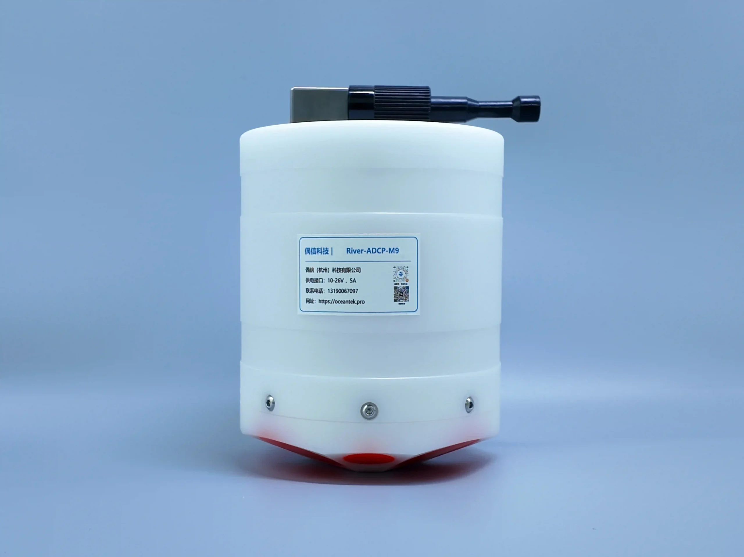
The River-ADCP-M9: Built-in Dual-Frequency in a Single Instrument
The Oceantek River-ADCP-M9 represents the most direct approach to dual-frequency ADCP operation: three frequencies integrated into a single 9-beam acoustic head. Designed for shallow-to-moderate-depth rivers, it eliminates the need for separate instruments while providing the benefits of multi-frequency profiling.
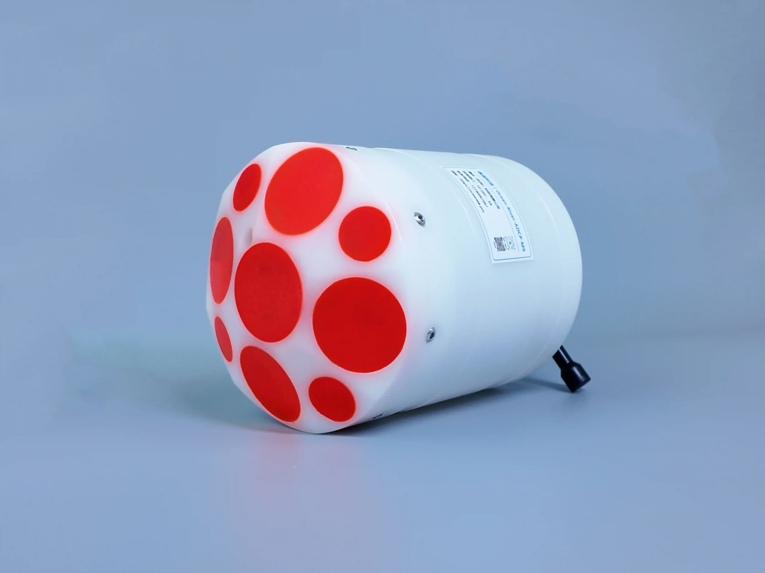
9-Beam Architecture Explained
The River-ADCP-M9’s acoustic head deploys three distinct beam groups simultaneously:
| Beam Group | Frequency | Quantity | Beam Angle | Primary Function |
|---|---|---|---|---|
| High-frequency Janus | 3.0 MHz | 4 beams | 25° | Shallow-water velocity profiling (0.06–0.8 m depth) |
| Mid-frequency Janus | 1.0 MHz | 4 beams | 25° | Mid-depth velocity profiling (0.8–40 m) |
| Vertical bathymetry | 0.5 MHz | 1 beam | 0° (nadir) | Echo sounding, channel bed survey, depth reference |
This architecture delivers gapless vertical coverage from 0.06 m to 40 m. At the shallow extreme—a 0.1 m deep headwater stream during drought—the 3.0 MHz beams maintain valid velocity data with cell sizes as fine as 0.02 m. At the deep end, the 1.0 MHz beams profile the full water column while the 0.5 MHz vertical beam simultaneously maps the channel bed to 80 m depth with 0.02% accuracy.
Key Specifications at a Glance
| Parameter | Specification |
|---|---|
| Beam Configuration | 9 beams: 4×3.0 MHz + 4×1.0 MHz + 1×0.5 MHz |
| Profiling Range | 0.06–40 m |
| Cell Size | 0.02–4 m (user-configurable) |
| Number of Cells | Up to 255 |
| Velocity Accuracy | ±0.25% ± 2 mm/s |
| Velocity Range | ±20.0 m/s maximum |
| Depth Measurement | 0.2–80 m (accuracy: 0.02%) |
| Bottom Tracking | 0.3–40 m |
| Data Output Rate | 2 Hz (internal sampling up to 70 Hz) |
| Internal Storage | 64 GB |
| Communication | RS-232, RS-422, GNSS/GPS input |
| Integrated Sensors | Temperature (±0.1°C), Pressure (±0.25%), Heading (0.8° RMS), Roll/Pitch (±1° RMS) |
| Weight (in air) | ≤1.5 kg |
| Depth Rating | 50 m |
| Operating Temperature | −5°C to 45°C |
At 1.5 kg, the River-ADCP-M9 is light enough for single-person deployment—wading, from a small unmanned surface vessel (USV-ADCP integration), or mounted on a portable frame. Its 50 m depth rating and 64 GB onboard storage support extended unattended operation at fixed monitoring stations.

Strategy 2: Multi-Instrument Dual-Frequency Deployment
For permanent gauging stations on large rivers—or sites requiring simultaneous fixed and mobile measurements—a two-instrument deployment with complementary frequencies offers advantages that even the best single-instrument solution cannot match:
Fixed H-ADCP + Vessel-Mounted Multi-Frequency ADCP
This is the most powerful configuration for continuous real-time discharge monitoring with periodic calibration. A fixed HADCP-600 (600 kHz horizontal ADCP) provides the index-velocity time series. Periodic surveys with the River-ADCP-M9 provide:
- High-resolution moving-boat discharge transects for index-velocity rating curve calibration and re-validation
- Detailed bathymetry via the 0.5 MHz vertical beam, updating cross-section geometry after flood events
- Near-boundary velocity data from the 3.0 MHz beams that the 600 kHz H-ADCP cannot resolve
- Independent quality control—discrepancies between the H-ADCP index velocity and the M9 transect-averaged velocity trigger investigation
This dual-instrument approach maps directly onto the best-practice calibration protocol described in our ADCP consistency test methodology.
Dual H-ADCP Deployment (300 kHz + 600 kHz)
At the Zhicheng hydrological station on the Yangtze River, researchers deployed 300 kHz and 600 kHz H-ADCPs simultaneously at different tilt angles along the same cross-section. The combined scheme delivered measurable accuracy gains over either instrument alone. This approach is appropriate when:
- The river width exceeds the reliable profiling range of a single 600 kHz unit
- Backwater or tidal effects create complex, multi-directional velocity fields
- Operational redundancy is required—if one instrument fails, the other maintains partial data continuity
- Suspended sediment varies widely enough that no single frequency maintains valid data across all conditions
Avoiding Acoustic Interference Between Instruments
When deploying two ADCPs simultaneously at the same site, same-frequency acoustic interference is a real concern. Two 600 kHz instruments transmitting into overlapping water volumes will degrade each other’s data quality. Three mitigation strategies are established:
- Frequency separation: Operate each instrument at a unique frequency band (e.g., Instrument A at 300 kHz, Instrument B at 600 kHz). This is the simplest and most robust approach.
- Spatial separation: Deploy instruments on opposite banks with non-overlapping beam paths—effective in channels wider than the combined profiling range of both instruments.
- Temporal interleaving: If same-frequency operation is unavoidable, stagger ping ensembles so that the two instruments never transmit simultaneously. This reduces the effective sampling rate by half but preserves data quality.
For permanent installations, consult Oceantek’s technical FAQ or contact engineering support at sales@oceanadcp.com for site-specific deployment planning.
Integrating Multi-Frequency Data Streams
Dual-frequency data brings a data-management challenge: two (or three) velocity profiles with different spatial resolutions must be merged into a single discharge estimate. Three integration strategies are in current practice:
1. Composite Profile Method
Build a single velocity profile by selecting the highest-quality data from each frequency in each depth bin. The 3.0 MHz beams dominate the upper water column; the 1.0 MHz beams take over at depth. The transition zone (typically 0.6–1.0 m depth, depending on turbidity) is where both frequencies overlap—this overlap zone provides built-in quality control: if the two frequencies disagree significantly at the same depth, either turbulence decorrelation or acoustic interference is indicated.
2. Weighted-Average Method
In the overlap zone, compute a signal-quality-weighted average of the two frequencies’ velocity estimates. Weighting factors are derived from per-cell correlation magnitude and percent-good ping counts. This approach maximizes the use of redundant data and reduces random uncertainty in the transition zone.
3. Independent Index-Velocity Method (Fixed Stations)
For permanent multi-frequency H-ADCP stations, build separate index-velocity rating curves for each frequency and compute discharge independently. The final discharge is the mean of the two estimates, with the difference between them serving as a real-time uncertainty indicator. When the two estimates diverge beyond a pre-set threshold (e.g., ±5%), an alert is triggered for operator review.
Calibration Considerations for Dual-Frequency Systems
Dual-frequency ADCP deployments introduce calibration complexities beyond single-frequency practice:
- Frequency-specific speed-of-sound correction: While sound speed in water is theoretically frequency-independent, the effective sound speed within an ADCP measurement volume can shift slightly with frequency in highly turbid water due to sediment-induced dispersion. When the two frequencies produce systematically different mean velocities in the overlap zone, verify the sound-speed input and consider a frequency-specific bias correction derived from moving-boat intercomparison.
- Per-frequency compass calibration: If deploying two physically separate instruments, calibrate each unit’s internal compass independently at the deployment site. Magnetic anomalies from mounting structures affect different instrument positions differently.
- Cell-alignment verification: When merging profiles from two instruments deployed at different ranges from the bank, ensure that the depth cells are registered to the same vertical datum (typically the water surface or channel thalweg). A 0.5 m vertical misalignment between profiles can introduce systematic discharge biases of 3–5%.
- Cross-validation during contrasting conditions: Validate the dual-frequency discharge against an independent reference (e.g., moving-boat ADCP transects or Price current-meter gaugings) under at least three distinct hydraulic regimes: low flow, medium flow, and near-bankfull.
Operational Case Studies
Case 1: Shallow Headwater Gauging — Single M9 Deployment
Scenario: A headwater tributary ranging from 0.15 m (baseflow) to 4.5 m (flood), with clear water (SSC < 50 mg/L at baseflow). A fixed gauging station is required.
Solution: A single River-ADCP-M9 mounted on a bank-installed frame, operating at all three frequencies. The 3.0 MHz beams handle baseflow conditions where even a 600 kHz unit would be nearly blind; the 1.0 MHz beams cover flood-stage profiling. The 0.5 MHz vertical beam provides continuous stage and bed-elevation monitoring, eliminating the need for a separate pressure transducer.
Case 2: Large Regulated River — H-ADCP + M9 Combination
Scenario: A 180 m wide regulated river with diurnal flow variations from upstream hydropower operations. Backwater effects from a downstream confluence during high flows.
Solution: A fixed HADCP-600 (600 kHz horizontal) on the left bank for continuous index-velocity monitoring. Monthly moving-boat surveys with the River-ADCP-M9 provide discharge calibration transects. The M9’s 9-beam architecture captures the full vertical velocity structure—including the near-bed velocities that the H-ADCP’s horizontal beams cannot see—improving the representativeness of the index-velocity rating. The combination achieves first-class hydrological station accuracy standards (<3% runoff volume error) under all flow conditions.
Case 3: Tidal Estuary — Dual H-ADCP
Scenario: A tidally influenced lower reach with bi-directional flow, salinity stratification, and channel width of 90 m.
Solution: Dual fixed H-ADCPs at 300 kHz and 600 kHz, deployed on the same bank at complementary tilt angles. The 300 kHz unit ensures profiling across the full channel width during high-turbidity ebb flows; the 600 kHz unit provides finer spatial resolution during lower-turbidity flood tides. Independent index-velocity ratings are maintained for each instrument, with the dual estimate providing real-time uncertainty bounds. The system achieves an R² of 0.99 for the combined discharge estimate.
Decision Framework: Which Approach for Your Site?
| Site Characteristics | Recommended Configuration | Key Instrument(s) |
|---|---|---|
| Shallow stream (<5 m), clear to moderate turbidity | Single dual-frequency instrument (fixed or survey) | River-ADCP-M9 |
| Medium river (5–50 m), stable hydraulics | Single fixed H-ADCP + periodic M9 calibration surveys | HADCP-600 + River-ADCP-M9 |
| Large river (>50 m), backwater/tidal influence | Dual H-ADCP (300 + 600 kHz) + periodic M9 calibration | Dual H-ADCP + River-ADCP-M9 |
| Highly variable SSC (clean to >10 kg/m³) | Dual-frequency fixed deployment (300 + 600 kHz) | Dual H-ADCP or dual-frequency instrument |
| Sediment flux monitoring as co-objective | Multi-frequency backscatter analysis (3+ frequencies) | River-ADCP-M9 + fixed H-ADCP |
| Budget-constrained, single-operator site | Single M9 for all survey + periodic gauging needs | River-ADCP-M9 |
Summary of Best Practices
- Match frequency to the dominant hydraulic challenge—shallow water demands high frequency; deep or turbid water demands low frequency. If both challenges exist at the same site, dual-frequency deployment is indicated.
- Use a built-in multi-frequency instrument (like the River-ADCP-M9) when the primary need is a single deployment platform covering a wide depth range—this simplifies logistics, data management, and calibration.
- Use separate instruments at different frequencies when redundancy, independent cross-validation, or complementary deployment geometries (horizontal vs. vertical beam orientation) are required.
- Avoid acoustic interference through frequency separation, spatial separation, or temporal interleaving. Same-frequency co-deployment without mitigation degrades both instruments’ data.
- Exploit the overlap zone—when two frequencies sample the same depth, use the redundant data for quality control and uncertainty estimation, not just for profile merging.
- Validate under contrasting conditions—a dual-frequency discharge model calibrated only at medium flow may perform poorly at extremes. Invest in calibration measurements across the full expected range.
- Maintain independent per-frequency metadata—track SNR, correlation, and percent-good separately for each frequency to enable rapid diagnosis when one frequency degrades.
Conclusion
Dual-frequency ADCP deployment is not a niche technique—it is increasingly the standard of practice for hydrological monitoring stations that face variable depth, turbidity, or hydraulic conditions. The physics are unambiguous: no single acoustic frequency can optimally profile every river state. The practical question is whether to achieve multi-frequency coverage through a single integrated instrument like the Oceantek River-ADCP-M9, or through a coordinated multi-instrument deployment.
The River-ADCP-M9’s 9-beam, triple-frequency architecture makes it the most streamlined path to dual-frequency capability for the majority of river monitoring applications—especially where shallow-water performance, single-operator deployment, and rapid survey turnaround are priorities. For large-river permanent stations, pairing a fixed H-ADCP with periodic M9 calibration surveys provides the best of both worlds: continuous real-time data with high-accuracy, high-resolution periodic validation.
For further guidance on instrument selection, deployment planning, or site-specific configuration, explore the Oceantek technical support portal, download product manuals, or browse the Oceantek news section for the latest field applications and product updates.
References and Further Reading
- Li, Y., et al. (2024). “Research on Real-Time Flow Online Monitoring Technology Using Multi-Angle Inclined Deployment of H-ADCPs.” DOAJ — Directory of Open Access Journals.
- Moore, S. A., Le Coz, J., Hurther, D., & Paquier, A. (2011). “On the Use of Horizontal ADCPs for Sediment Flux Measurements in Rivers.” IAHR Congress Proceedings.
- Li, Y., et al. (2025). “Deep Characteristic Learning Model for Real-Time Flow Monitoring Based on H-ADCP.” Water Resources Research.
- Wang, J., & Chen, J. (2025). “H-ADCP-Based Online Discharge Monitoring Model Using Feature Adaptive Optimization.” Journal of Hydrology.
- Nihei, Y., & Kimizu, A. (2007). “A New Discharge Monitoring System Using H-ADCP and a Data Assimilation Technique.” River Flow 2007.
- ISO 748:2007. Hydrometry — Measurement of liquid flow in open channels using current-meters or floats.
- ISO/TS 24154:2005. Hydrometry — Measuring river velocity and discharge with acoustic Doppler profilers.
- Oceantek. (2026). ADCP Equipment Consistency Test Report.
- Oceantek. (2026). Chinese ADCP Manufacturer Selection Guide.
- Oceantek. (2026). USV-ADCP: How Unmanned Boats Are Revolutionizing Intelligent River Monitoring Operations.
Disclaimer: Product specifications are subject to change. Always refer to the official River-ADCP-M9 product page for the latest technical data. Deployment decisions should be informed by site-specific hydrological assessment and professional engineering judgment.