If you ask an experienced hydrographer what the single most important ADCP specification is, they will not say accuracy, beam count, or brand. They will say frequency. Choose the wrong frequency, and your data will be either too coarse to resolve the features you care about, or collected from an instrument that cannot reach the bottom. This is not a decision you can fix with post-processing — frequency is baked into the transducer hardware, and switching means buying a different instrument.
The 300kHz versus 600kHz decision is the most common fork in the road for ADCP buyers. Between them, these two frequencies cover roughly 80% of all ADCP deployments worldwide. But the difference between them is not incremental — it is a fundamental physical trade-off that determines what your instrument can and cannot measure. This article explains the physics behind the choice, provides practical selection criteria, and includes real-world deployment examples so you can make the decision with confidence.
The Physics: Why Frequency Dictates Everything
Acoustic signals attenuate — lose energy — as they travel through water. The critical relationship is that attenuation increases with the square of the frequency. A 600kHz signal loses energy roughly four times faster than a 300kHz signal traveling through the same water. This is not a manufacturing limitation or a design compromise; it is a law of physics. The practical consequence is straightforward: lower-frequency sound travels farther before scattering back to the transducer with enough strength to be measured.
But the physics cuts both ways. To achieve the same range resolution, a lower-frequency ADCP must transmit a longer acoustic pulse. A longer pulse means a larger sampling volume — the instrument is averaging velocity over a bigger chunk of water. This is why lower-frequency ADCPs have larger minimum cell sizes. You simply cannot have a 0.25-meter depth cell at 300kHz with the signal-to-noise ratio required for accurate velocity measurement.
In practical terms, the trade-off is this: a 300kHz ADCP typically profiles to 150–200 meters with cell sizes of 1–4 meters. A 600kHz ADCP profiles to 60–80 meters with cell sizes of 0.5–2 meters. The choice comes down to whether your application prioritizes depth range or spatial detail. There is no instrument that gives you both at the same time, regardless of manufacturer or price.
There is a third factor that many buyers overlook: power consumption. Because a 300kHz signal attenuates more slowly, the transducer requires less transmit power to achieve the same range. For the same battery capacity, a 300kHz ADCP will typically run 30–50% longer than a 600kHz unit at the same sampling rate. In long-term autonomous deployments — think six-month moorings with no possibility of battery replacement — this difference can determine whether your deployment succeeds or comes back with three months of data followed by three months of silence.
When to Choose 300kHz
300kHz is the right frequency when your water depth exceeds 60–80 meters. This covers a broad range of applications: continental shelf current profiling, deep-water mooring deployments, offshore engineering surveys, and oceanographic research where you need the full water column from a single instrument. If your site map shows depths of 100 meters or more for any significant portion of your survey area, 300kHz is the only practical choice — a 600kHz unit will not reach the bottom, and you will have a gap in your velocity profile that no amount of data processing can fill.
Beyond raw range, 300kHz offers two operational advantages that matter in the field. First, lower-frequency sound is less sensitive to suspended sediment and biological scatterers — the small particles and plankton that reflect acoustic energy back to the transducer. In turbid coastal waters or during phytoplankton blooms, a 300kHz signal is more likely to maintain a usable profile than a 600kHz signal, which attenuates faster in particle-rich water. Second, the longer deployment endurance from lower power consumption makes 300kHz the default choice for autonomous moorings where battery life is the limiting factor.
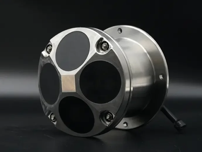
The Oceantek ADCP-300-DR-FA4 is purpose-built for these scenarios.
Real-world example: a national oceanographic agency monitoring the continental shelf break at 180 meters depth. A 600kHz ADCP would profile roughly the top third of the water column. A 300kHz unit captures the full profile from surface to seabed, providing the vertically complete current data that the agency’s circulation models require. The choice is not about which instrument is “better” — it is about which one actually answers the measurement question.
When to Choose 600kHz
600kHz is the workhorse frequency for most coastal, estuarine, and river applications. If your water depth is consistently under 70 meters — which covers the vast majority of river gauging stations, harbor monitoring setups, coastal engineering surveys, and aquaculture site assessments — 600kHz gives you finer spatial resolution without sacrificing the range you need. The smaller cell sizes (down to 0.5 meters, and in some configurations 0.25 meters) let you resolve current structure that a 300kHz instrument would blur across its coarser depth bins.
The finer resolution matters more than most users realize. Consider a river discharge measurement: the velocity gradient near the bed — where friction slows the flow — contains critical information for estimating bed roughness and calculating total discharge. A 300kHz ADCP with 2-meter cells might capture this gradient in two or three depth bins. A 600kHz unit with 0.5-meter cells captures it in eight to twelve bins. The discharge calculation from the 600kHz data will be measurably more accurate, particularly in channels where the flow is sheared or stratified.
The Oceantek ADCP-600-DR-FA4 is the most popular instrument in our product line specifically because it covers so many common deployment scenarios. In direct-reading mode with a surface cable, it provides real-time velocity profiles for vessel-mounted surveys and fixed monitoring stations. The 600kHz frequency hits the sweet spot for the depth ranges that most users actually work in.
Real-world example: a port authority conducting a current survey for navigation safety in a 45-meter-deep harbor approach channel. A 300kHz ADCP would profile the water column but with 2-meter cells that might miss thin shear layers affecting vessel handling. A 600kHz unit with 0.5-meter cells resolves those features, giving the harbor pilots a more accurate picture of what currents to expect at each depth. The instrument reaches the bottom with margin to spare, so range is not the constraint — resolution is.
What About Other Frequencies?
The 300kHz/600kHz decision covers most scenarios, but it is worth knowing where the other standard frequencies fit so you can rule them in or out with confidence.
75kHz instruments profile to 500–700 meters and are used for full ocean-depth work — basin-scale circulation studies, deep-water current monitoring for offshore oil and gas, and abyssal oceanography. If your site is deeper than 200 meters, you should be looking at 75kHz, not 300kHz. These are specialized, expensive instruments, and they are overkill for any application in less than 150 meters of water.
1200kHz ADCPs profile to about 15–25 meters with cell sizes as small as 0.1–0.25 meters. They are the right choice for very shallow rivers, small streams, laboratory flumes, and near-bed boundary layer studies where centimetric resolution is the overriding requirement. If your deepest expected water is under 20 meters and you need to resolve velocity structure within a few centimeters of the bed, 1200kHz is worth evaluating.
3000kHz instruments are niche tools for laboratory use, extremely shallow streams (under 5 meters), and research applications demanding the finest possible spatial resolution — cell sizes down to a few centimeters. For most field applications, 3000kHz is unnecessary and its very limited range makes it unsuitable for anything but the shallowest environments.
For guidance on frequency selection across the full spectrum, including how frequency interacts with other parameters like beam angle and transducer configuration, see our complete ADCP parameter selection guide.
The Decision Framework: Three Questions to Ask
You can narrow the frequency decision to three questions. Answer them honestly, and the right choice will be clear:
1. What is the maximum water depth at your site? Not the average depth — the maximum depth you need to profile. If it exceeds 80 meters, the decision is made: you need 300kHz (or 75kHz if over 200 meters). A 600kHz unit will not reach the bottom, and an incomplete profile is worse than a coarse one. If your maximum depth is under 70 meters, continue to the next question.
2. What is the smallest current feature you need to resolve? This is the harder question because it requires you to think about your data product, not just your deployment site. Are you measuring mean discharge for a hydrological record? 2-meter cells at 300kHz are probably fine. Are you studying shear-driven mixing in an estuary? You need the 0.5-meter resolution that 600kHz provides. Are you measuring turbulence parameters? Neither frequency will do — you need an ADV, not an ADCP (see our instrument comparison resources). Be honest about the resolution your analysis actually requires, not the resolution that sounds impressive.
3. Is your deployment autonomous (power-constrained) or cabled (power-unlimited)? If you are deploying on a mooring for six months with no way to change batteries, the power efficiency advantage of 300kHz may outweigh the resolution advantage of 600kHz — even if your site is within 600kHz range. If you have shore power or can swap batteries weekly, power is not a constraint, and 600kHz becomes the natural choice for its finer resolution.
If, after answering these three questions, you find that both range and resolution matter equally for your project — perhaps you are surveying across a sharp depth gradient, from a shallow shelf into deep water — consider deploying two instruments at different frequencies. The cost of a second ADCP is often less than the cost of redoing a field campaign with the wrong instrument. Many major oceanographic programs run 300kHz for deep-water coverage and 600kHz for shallow-water detail simultaneously.
A Note on Water Clarity and Scatterers
All acoustic Doppler instruments depend on particulate matter in the water to reflect sound back to the transducer. In exceptionally clear water — oligotrophic open-ocean environments, for example — there may be insufficient scatterers to produce a strong return signal, and the effective profiling range of any frequency will be reduced. This affects higher frequencies more severely because of their faster attenuation rate. If you work in very clear water, factor in a 20–30% range reduction from the manufacturer’s specification, and consider whether 300kHz’s longer range buys you margin against low-scatterer conditions that a 600kHz unit would not have.
The reverse is also true: in highly turbid water with abundant suspended sediment, signal attenuation increases, and the effective range of both frequencies drops. Here, the 300kHz instrument’s slower attenuation rate again provides a buffer that the 600kHz unit lacks. If your site is both turbid and relatively deep (50–80 meters), 300kHz may be the safer choice even though 600kHz nominally covers that depth range.
The frequency decision is not just about depth on a chart — it is about the acoustic environment you are actually operating in. The best specification in the world means nothing if the sound never reaches the scatterers and makes it back to the receiver.
Browse Oceantek ADCP products across all frequency ranges to find the instrument matched to your specific deployment conditions.