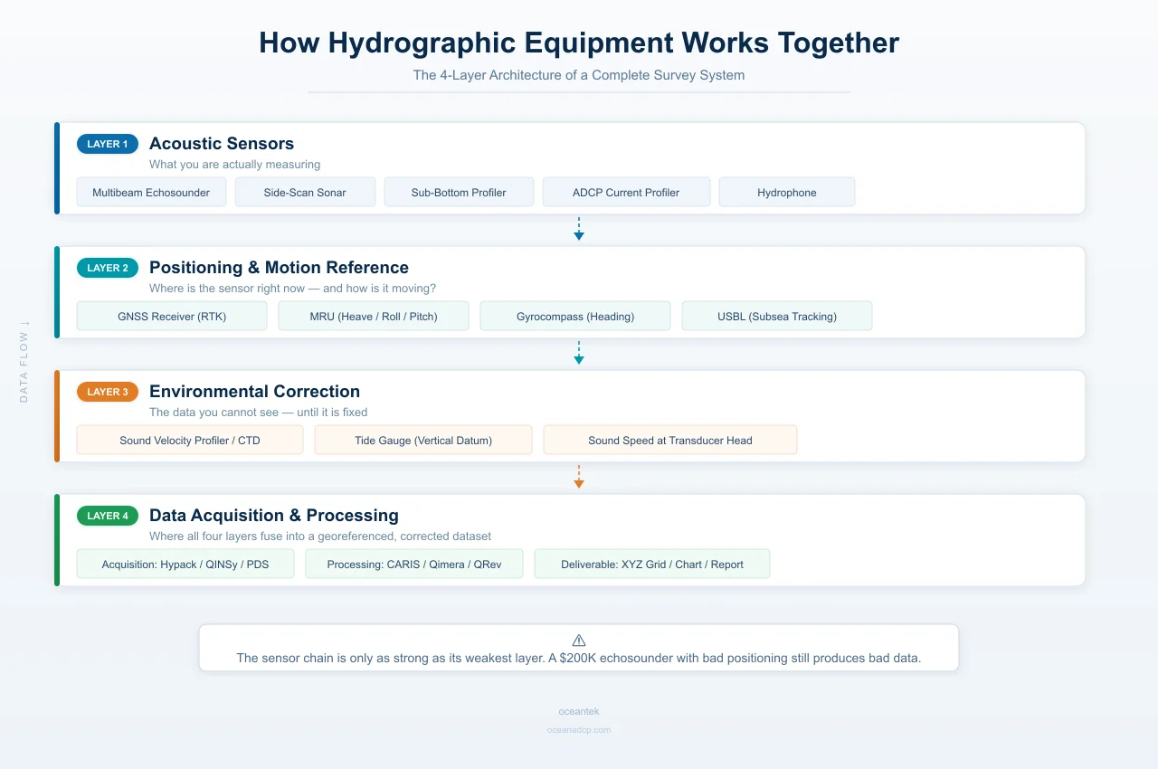
A hydrographic survey is a chain of four interdependent systems: acoustic sensors, position references, environmental correctors, and data processors. If any link in that chain is misconfigured — a sound velocity profile two hours out of date, an MRU lever arm measured wrong by 50 centimeters — every depth measurement that follows is wrong. The instruments are all working perfectly. The data is garbage.
Table of Contents
- 1. The 4-Layer Architecture of a Hydrographic Survey System
- 2. A Day on a Survey Vessel: Equipment in Action
- 3. The Most Common Integration Mistakes
- 4. How the Equipment Stack Changes by Project
- 5. The Shift to Unmanned Platforms
- 6. Frequently Asked Questions
1. The 4-Layer Architecture of a Hydrographic Survey System
Every piece of hydrographic equipment on a survey vessel belongs to one of four functional layers. Understanding these layers — and the data dependencies between them — is the difference between a clean dataset and one that fails QA:
Layer 1: Acoustic Sensors — What You Are Actually Measuring
This is the layer most people think of as “hydrographic equipment.” These instruments transmit acoustic energy into the water and measure what comes back:
- Multibeam Echosounder (MBES) — Transmits a fan of acoustic beams and measures the two-way travel time and angle of each return. Produces a swath of depth measurements. The core sensor for any bathymetric survey.
- Side-Scan Sonar — Transmits a narrow fan-shaped beam to each side and records the intensity of seabed backscatter. Produces an acoustic image of the seafloor texture — think black-and-white aerial photography, but with sound.
- Sub-Bottom Profiler (SBP) — Uses lower frequencies (2–15 kHz) that penetrate the seabed and reflect off sediment layer boundaries. Produces a cross-section of subsurface geology.
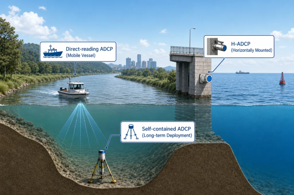
- ADCP — Measures water current velocity at multiple depths simultaneously. Critical for understanding flow conditions during survey operations and — on DP vessels — providing real-time current input to the dynamic positioning system.
Key point: No acoustic sensor produces usable data without the next three layers. The raw acoustic returns are meaningless until they are positioned, corrected, and integrated.
Layer 2: Positioning and Motion — Where Is the Sensor Right Now?
An echo sounder knows how deep the water is below the transducer. It has no idea where that depth measurement is on the Earth’s surface. That job belongs to the positioning layer:
- GNSS Receiver — Provides the vessel’s absolute position. Accuracy ranges from sub-meter (standard code-based) to centimeter-level (RTK or PPK with a base station or correction service). For hydrographic surveys requiring IHO Special Order accuracy, RTK-grade GNSS is mandatory.
- Motion Reference Unit (MRU) — Measures vessel roll, pitch, heave, and heading. This is not optional. A 5° roll on a vessel in 30 m of water creates a lateral depth error of approximately 2.6 m at the outer beams of a multibeam swath. The MRU corrects for this by reporting the instantaneous orientation of the transducer head.
- Gyrocompass / AHRS — Provides true heading. Combined with the MRU, this allows the acquisition software to compute the exact position and orientation of every acoustic beam on the seafloor.
The critical relationship: Positioning accuracy is the ceiling on your survey accuracy. A $200,000 multibeam echosounder feeding data into a $2,000 GNSS receiver without an MRU will produce worse bathymetry than a $20,000 single-beam with proper positioning. The sensor chain is only as strong as its weakest layer.
Layer 3: Environmental Correction — The Data You Cannot See Until It Is Fixed
Sound does not travel in straight lines underwater — it bends. It also changes speed with temperature, salinity, and pressure. If you do not correct for these effects, your bathymetry data will contain systematic errors that look plausible but are wrong:
- Sound Velocity Profiler (SVP) / CTD — Measures the speed of sound as a function of depth. This profile is used to ray-trace every multibeam beam: computing the actual curved path the acoustic pulse traveled through the water column. Without a sound velocity profile, the MBES assumes sound travels in straight lines at a constant speed — which it never does.
- Tide Gauge — Measures water level change over time. All depth measurements must be reduced to a common vertical datum (usually Chart Datum or Mean Sea Level). A 3-meter tidal range that is not corrected produces a 3-meter depth error.
How often to measure: Sound velocity profiles should be collected at minimum once per survey day, and immediately whenever the vessel crosses a water mass boundary (river plume, tidal front, thermocline). A profile that was valid at 8 AM may be wrong by noon.
Layer 4: Data Acquisition and Processing — Where It All Comes Together
This layer takes raw data from Layers 1–3 and fuses it into a coherent survey dataset:
- Acquisition Software (Hypack, QINSy, Teledyne PDS) — Receives real-time data streams from every sensor. Applies positioning offsets, motion compensation, sound velocity correction, and tide reduction. Displays the processed bathymetry in real time so the surveyor can see coverage and flag anomalies.
- Post-Processing Software (CARIS, Qimera, QRev) — Refines the dataset after acquisition. Removes outliers, applies statistical filters, verifies sound velocity and tide corrections, and produces final deliverables (XYZ grids, contours, volume calculations).
Data flow in one sentence: Acoustic travel times (Layer 1) + positions and attitudes (Layer 2) + sound speed and tide corrections (Layer 3) → fused in real time (Layer 4) → a georeferenced, corrected digital model of the seafloor.
2. A Day on a Survey Vessel: Equipment in Action
Technical diagrams are useful. But they do not capture what it actually feels like to run a hydrographic survey. Here is a real operational sequence — a typical 12-hour survey day — showing how the equipment layers interact in practice.
06:30 — Pre-Survey Checks
The surveyor arrives at the vessel and powers up the acquisition laptop. Before leaving the dock, she runs through a checklist:
- GNSS receiver locked? Fix type RTK? — Check.
- MRU initialized and reporting stable heave? — Check.
- MBES online, all beams transmitting, no errors in the diagnostic window? — Check.
- Sound velocity probe calibrated and ready for a cast? — Check.
A 15-minute pre-survey check prevents hours of bad data. The most experienced surveyors treat this step as non-negotiable — they have been burned before.
07:15 — Sound Velocity Cast
The vessel steams to the survey area. Before any bathymetry is collected, the surveyor deploys the SVP over the side. The probe descends at roughly 1 m/s, measuring sound speed every centimeter. The profile shows a strong thermocline at 18 meters: sound speed drops from 1,520 m/s to 1,485 m/s over a 5-meter band. Without this profile, every MBES beam passing through that layer would refract — and every depth measurement below 18 meters would be systematically wrong.
The profile is loaded into the acquisition software. The ray-tracing engine now has the information it needs to compute true beam paths.
08:00 — Survey Lines Begin
The vessel runs parallel survey lines at 100-meter spacing. On the acquisition display, the surveyor watches three things simultaneously:
- Coverage map — Is each swath overlapping the previous one by at least 20%?
- Waterfall display — Are the outer beams noisy? If beam intensity drops off at the edges, the swath width may need to be reduced.
- GNSS age — Is the position latency under 0.1 seconds? A 1-second delay between position fix and depth measurement at 5 knots vessel speed creates a 2.5-meter horizontal error.
10:30 — ADCP Current Check
The vessel crosses a tidal front. The surveyor notices the outer MBES beams showing increased noise — the sound velocity is changing across the front. She deploys the ADCP to measure the current structure, confirming a 0.8 m/s shear across the front. A second SVP cast is taken on the other side. The new profile is 4 m/s faster at the surface than the morning cast — enough to create noticeable depth artifacts if uncorrected.
14:00 — Side-Scan Target Investigation
During a lunch break review of the side-scan mosaic, the surveyor spots an acoustic shadow on the seabed — a linear feature 12 meters long, not charted. She marks the position, deviates from the survey plan, and runs two higher-resolution passes over the target. The side-scan imagery reveals a lost container. Position, dimensions, and orientation are logged. The client’s environmental team will need this.
17:30 — End of Day Processing
Back at the dock, the surveyor runs automated cleaning on the day’s MBES data. She checks the tide gauge record to confirm the tide correction matches the observed water level. She applies the afternoon SVP profile to the post-13:00 data. The cleaned dataset shows 98.7% coverage of the planned area with one small gap in the southwest corner — noted for infill tomorrow.
This is what a functioning 4-layer system looks like. Every instrument did its job — because they were integrated correctly.
3. The Most Common Integration Mistakes
Hydrographic equipment failures rarely happen because an instrument breaks. They happen because two correctly-functioning instruments are set up to talk to each other incorrectly. Here are the integration errors that surveyors encounter most often — and how to prevent them.
Mistake 1: Sound Velocity Profile Too Old
What happens: The surveyor takes one SVP cast at the start of the day and uses it for 10 hours of survey work across multiple water masses. The acquisition software ray-traces every beam with a profile that no longer matches reality. The result: the outer beams of the swath — which travel at the steepest angles and traverse the most water — develop a characteristic “smile” or “frown” depth artifact. The data looks smooth but is wrong by 0.5–2% of water depth at the swath edges.
How to prevent it: Deploy the SVP whenever the vessel crosses a known water mass boundary, whenever the surface sound speed changes by more than 2 m/s, and at minimum every 4 hours. An underway sound velocity probe that can be deployed without stopping the vessel pays for itself in data quality.
Mistake 2: MRU Lever Arm Not Measured
What happens: The MRU is installed in a convenient location — a deck box, a cabin — but its position relative to the MBES transducer head (the “lever arm”) is not accurately measured. When the vessel rolls, the acquisition software compensates for the MRU’s motion and applies that correction to the transducer — but the geometry is wrong. A 50 cm error in lever arm measurement creates meter-scale depth errors at the outer beams.
How to prevent it: Measure the 3D offset between the MRU and the transducer reference point with a total station or tape, to within 1 cm accuracy. Enter these values into the acquisition software’s vessel configuration file. Re-measure if the MRU or transducer is ever moved.
Mistake 3: GNSS Latency Unaccounted For
What happens: The GNSS receiver outputs position at 10 Hz. The MBES pings at 20 Hz. Between each GNSS fix, the vessel has moved — at 5 knots, roughly 12 cm per 50-millisecond interval. If the acquisition software does not time-tag and interpolate positions correctly, every depth point carries a position error proportional to vessel speed × latency.
How to prevent it: Verify that the acquisition software displays “GNSS age” — the time since the last valid position fix — and confirm it stays under 0.1 seconds. Use a 1-PPS (pulse-per-second) timing signal from the GNSS to synchronize all sensor clocks. This is standard on survey-grade GNSS receivers but often overlooked in setup.
Mistake 4: Acoustic Interference Between Instruments
What happens: The MBES operates at 200–400 kHz. The ADCP operates at 300 kHz. When both transmit simultaneously, the ADCP’s acoustic pulses are received by the MBES as noise — and vice versa. The result: degraded data quality on both instruments, with no obvious cause unless the operator knows to check for frequency overlap.
How to prevent it: Check the operating frequencies of every acoustic instrument before the survey. If two instruments share overlapping bands, either separate them in time (alternating pings) or physically — mounting the ADCP on the opposite side of the vessel from the MBES, or using a deeper pole mount to increase acoustic separation.
4. How the Equipment Stack Changes by Project
There is no single “correct” set of hydrographic equipment. The stack changes based on what you are measuring, how precise you need to be, and what the client’s deliverable requires:
| Project Type | Core Equipment | Supporting Instruments | Why This Stack |
|---|---|---|---|
| Navigation Channel Dredging Survey | Single-beam echosounder + RTK GNSS + MRU | Tide gauge, CTD | Depth accuracy is the only requirement. Single-beam is sufficient for channel cross-sections. RTK GNSS eliminates the need for post-processed tide correction if ellipsoid-referenced. |
| Offshore Wind Farm Site Survey | MBES + Side-scan sonar + ADCP + MRU | SVP, SBP, magnetometer (UXO clearance) | Full seabed characterization required: bathymetry (MBES), seabed texture and objects (side-scan), sub-seabed geology (SBP), currents for foundation design (ADCP), unexploded ordnance (magnetometer). |
| Pipeline Route Inspection | MBES + Side-scan sonar + USBL | SBP, CTD | Pipeline burial depth (SBP), free spans (MBES profile), damage/encroachment (side-scan). USBL tracks the ROV or towfish position precisely along the pipeline route. |
| Environmental Baseline Study | CTD + ADCP + Hydrophone | Dissolved oxygen sensor, turbidity sensor, water sampler | Not a bathymetric survey. Focus is water column characterization: temperature/salinity structure (CTD), current regime (ADCP), ambient noise and marine mammal presence (hydrophone). Builds the pre-construction environmental baseline. |
| Wreck Search and Salvage | MBES + Side-scan sonar + Magnetometer | USBL, ROV with camera | Wide-area search with side-scan + magnetometer (ferrous targets). High-resolution MBES once the target is located. ROV with USBL tracking for visual confirmation. |
| River Discharge Monitoring Station | H-ADCP (horizontal) + Stage gauge | Telemetry (4G/satellite), solar power system | Continuous, unattended monitoring. H-ADCP measures velocity at a fixed horizontal layer. Stage gauge provides water level. Discharge is computed from the index-velocity relationship. No vessel required after installation. |
The pattern: start with what you need to measure, then add the sensors that make that measurement accurate, then add the correctors that remove systematic errors. Never start with a list of equipment and work backwards.
5. The Shift to Unmanned Platforms
The most significant change in hydrographic equipment over the last decade is not a new sensor type. It is the platform carrying the sensors: Unmanned Surface Vessels (USVs) and Autonomous Underwater Vehicles (AUVs) are replacing manned survey vessels for a growing range of applications.
This shift is reshaping equipment design requirements:
Smaller, Lighter, Less Power
A manned survey vessel can carry a 40 kg multibeam transducer head without concern. A USV with a 25 kg payload budget cannot. Equipment manufacturers are responding with compact, integrated sensor heads: the multibeam, INS, and sound velocity probe in a single housing. Phased-array transducers — flat ceramic plates with electronic beam steering — are replacing piston transducers because they fit into smaller form factors without sacrificing beam count.
Autonomous Operations Require Autonomous QC
On a manned vessel, the surveyor watches the waterfall display and flags bad data. On a USV operating 5 km from the mother vessel, nobody is watching. The acquisition software must now include automated quality control: detecting when outer beams are noisy, flagging sound velocity anomalies, and alerting the remote operator — or adjusting survey parameters automatically. This capability is still maturing, and it will separate the next generation of survey equipment from the current one.
Integration Moves to the Factory
Historically, the survey company integrated the equipment: buying a sonar from one manufacturer, a GNSS from another, an MRU from a third, and making them work together. With unmanned platforms, much of this integration is moving to the factory. A USV arrives with sensors pre-installed, offsets pre-measured, and calibration pre-verified. This reduces setup time from days to hours — but it also means the surveyor must trust the manufacturer’s integration, which places a premium on working with manufacturers who have in-house sensor expertise, not just platform integrators.
This trend does not mean surveyors will be replaced. It means the surveyor’s role shifts from equipment operator to data quality manager: planning the mission, monitoring automated QC, and making the judgment calls that software cannot. The equipment becomes more autonomous; the surveyor becomes more strategic.
6. Frequently Asked Questions
There is no single most important instrument — and that is the point of this article. A hydrographic survey is a system. The multibeam echosounder gets the attention because it produces the bathymetry, but without a properly configured GNSS receiver, a calibrated MRU, and a valid sound velocity profile, that multibeam data is unusable. If forced to name the most overlooked instrument, it would be the motion reference unit — many surveyors underestimate how much depth error vessel motion introduces until they see the before-and-after comparison with MRU correction applied.
At minimum: once at the start of the survey day, and again whenever the vessel crosses a known water mass boundary (estuary plume, tidal mixing front, major current boundary). A practical rule: if the surface sound speed has changed by more than 2 m/s since the last cast, take another profile. For surveys covering large areas with varying water masses, an underway sound velocity profiler that can be deployed without stopping the vessel is a worthwhile investment — it pays for itself in reduced re-survey time.
Hydrographic equipment is primarily concerned with measuring the shape and nature of the seafloor: bathymetry, seabed imagery, and sub-bottom structure. Its primary output is nautical charts, seabed maps, and engineering survey deliverables. Oceanographic equipment is primarily concerned with measuring water column properties: currents, temperature, salinity, and acoustics. Its primary output is scientific data for understanding ocean processes.
In practice, the boundary blurs. An ADCP is oceanographic equipment when used to study circulation patterns, and hydrographic equipment when used to provide real-time current data to a DP vessel during a survey. A CTD is used by both disciplines — hydrographers for sound speed correction, oceanographers for water mass analysis. Most survey vessels carry equipment from both categories.
On a small vessel with modern integrated equipment: yes. A single surveyor can manage the acquisition software, monitor data quality, deploy the SVP, and make survey decisions — provided the system is properly set up and calibrated beforehand. This is increasingly common for nearshore and inland surveys using compact USVs or small survey launches. For large offshore surveys with multiple simultaneous sensors (MBES + side-scan + SBP + ADCP), a two-person survey team is more typical: one running acquisition, one monitoring data quality and planning line adjustments.
The standard workflow uses two types of software. Acquisition software (Hypack, QINSy, Teledyne PDS, BeamworX) runs during the survey: it receives real-time sensor data, applies corrections, displays coverage, and logs raw data. Post-processing software (CARIS HIPS/SIPS, Qimera, QRev for ADCP discharge, MB-System for open-source workflows) runs after the survey: it cleans outliers, verifies corrections, and produces final deliverables. Some surveys also use GIS software (ArcGIS, QGIS) for final map production and data management. For a small survey operation starting out, Qimera and QRev are common entry points — Qimera handles MBES processing, QRev handles ADCP discharge computations, and both are widely used in the industry.
Planning a Hydrographic Survey?
Oceantek manufactures ADCPs, DVLs, and hydrophones — the current measurement and acoustic monitoring components of a complete hydrographic system. If you are building or upgrading a survey system and need advice on instrument selection, our engineering team can help.
- ✅ Free technical consultation — tell us your survey objectives and depth range
- ✅ Instrument datasheets and comparison test reports available
- ✅ Direct manufacturer pricing for ADCP, DVL, and hydrophones
- ✅ Integration support — we can verify protocol compatibility with your acquisition software
Contact Our Engineering Team →
Further Reading
- How Does an Acoustic Doppler Current Profiler Work? — Full Technical Guide
- Marine Survey Equipment Selection Guide: A Practical Buyer’s Framework
- What Is a DVL? Difference Between DVL and ADCP
- Bottom-Tracking vs Water-Tracking in DVL: How It Works
- Planning a Bankable Metocean Current Measurement Campaign for Offshore Wind
- DVL Buyer’s Guide for AUV/ROV Navigation