Table of Contents
- Why Water Flow Measurement Is Harder Than You Think
- The Water Flow Measurement Landscape: A Map, Not a List
- Open Channel Methods: From a Leaf to a Laser
- Closed Pipe Methods: When Water Travels Under Pressure
- The Accuracy Trap: Why ±1% Doesn’t Mean What You Think
- ADCP: The Method That Changed the Game
- Your Decision Framework: From “What Should I Use?” to “I Know What to Buy”
- The Future of Water Flow Measurement
- Quick Reference: Standards and Formulas
- Frequently Asked Questions
1. Why Water Flow Measurement Is Harder Than You Think
Let’s start with an uncomfortable truth: even experienced engineers get flow measurement wrong. A lot. We’ve seen a consulting firm install a ±0.5% electromagnetic flow meter three pipe-diameters downstream of a 90° elbow and wonder why their readings were off by 15%. We’ve watched a well-intentioned field tech use a float test on a wind-chopped reservoir and report “precise” numbers to three decimal places.
The instrument wasn’t the problem. The understanding was.
Here’s what most guides won’t tell you upfront: water flow measurement has three hidden challenges that no instrument can solve on its own.
Challenge 1: The velocity profile is never uniform
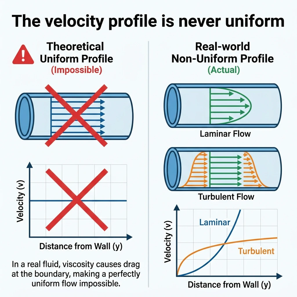
In an open channel, water at the surface moves faster than water near the bed. In a pipe, the velocity peaks at the center and drops to near-zero at the walls. If you measure at one point and assume the rest, you’re not measuring flow — you’re making an educated guess. The more turbulent or irregular the channel, the worse the guess.
Challenge 2: You change what you’re trying to measure
Put a current meter in the water, and it disturbs the flow around it. Install a weir, and it backs up water upstream. Insert an orifice plate, and you’ve permanently sacrificed pressure head. This is the fundamental tension between intrusive and non-intrusive methods — and it’s a choice every measurement campaign has to confront.
Challenge 3: One measurement is a snapshot, not a story
Flow changes minute to minute, season to season. The number you capture at 10:00 AM Tuesday says little about Wednesday afternoon, let alone next month’s flood. The real question isn’t “what’s the flow right now?” — it’s “how do I build a system that tells me what I need to know, when I need to know it?”
Key Insight: Most measurement guides start with instruments. We’re starting from the water itself — because the river, pipe, or ocean current doesn’t care which meter you bought. It will behave exactly as physics dictates, and your job is to understand enough physics to pick the right tool for this particular water, in this particular place, for this particular purpose.
2. The Water Flow Measurement Landscape: A Map, Not a List
Open ten guides on water flow measurement and nine of them will give you a list. “Here are 15 methods. Good luck.”
A list is useless when you don’t know what you’re looking for. So instead of a list, here’s a map. Two questions put you in the right neighborhood immediately:
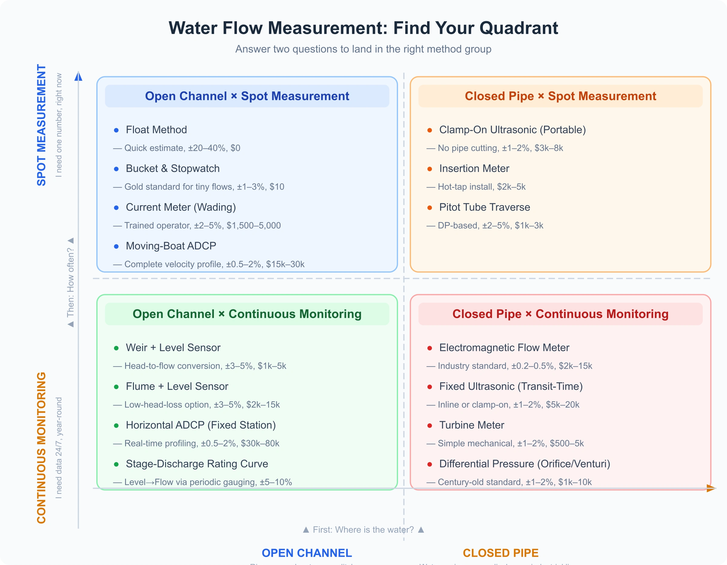
How to use this map: Locate your scenario. If you’re measuring an irrigation canal twice a year to calibrate water allocation, you’re in the top-left: Open Channel + Spot Measurement. If you’re running a municipal water treatment plant that needs real-time flow data for regulatory compliance, you’re in the bottom-right.
The rest of this guide is organized around getting you from “which quadrant am I in?” to “this is the specific instrument and installation method I need.”
Key Insight: The single most expensive mistake in flow measurement is choosing a method designed for the wrong quadrant. An instrument perfect for spot measurements in rivers will fail miserably — and expensively — when you try to adapt it for permanent pipe monitoring. Start with where and how often, then choose what.
3. Open Channel Methods: From a Leaf to a Laser
Open channel flow is the most common and most deceptively difficult measurement scenario. The surface is free, the geometry is irregular, and the bed is constantly shifting. Here’s every method worth knowing, ranked not by technology level but by when you’d actually use it.
3.1 The Float Method: When Good Enough Is Actually Good Enough
What it is: You time a floating object over a known distance, multiply by a correction factor, and multiply by cross-sectional area. That’s it.
Best for: A farmer who needs to know if the ditch is delivering roughly 50 or roughly 500 liters per second. A field biologist who needs a ballpark streamflow for a habitat assessment. An engineer doing a preliminary site visit with nothing but a tape measure and a phone stopwatch.
Accuracy reality: ±20% to 40% in practiced hands. Worse in wind, turbulence, or irregular channels. Surface velocity × 0.85 = mean velocity is a rule of thumb, not physics.
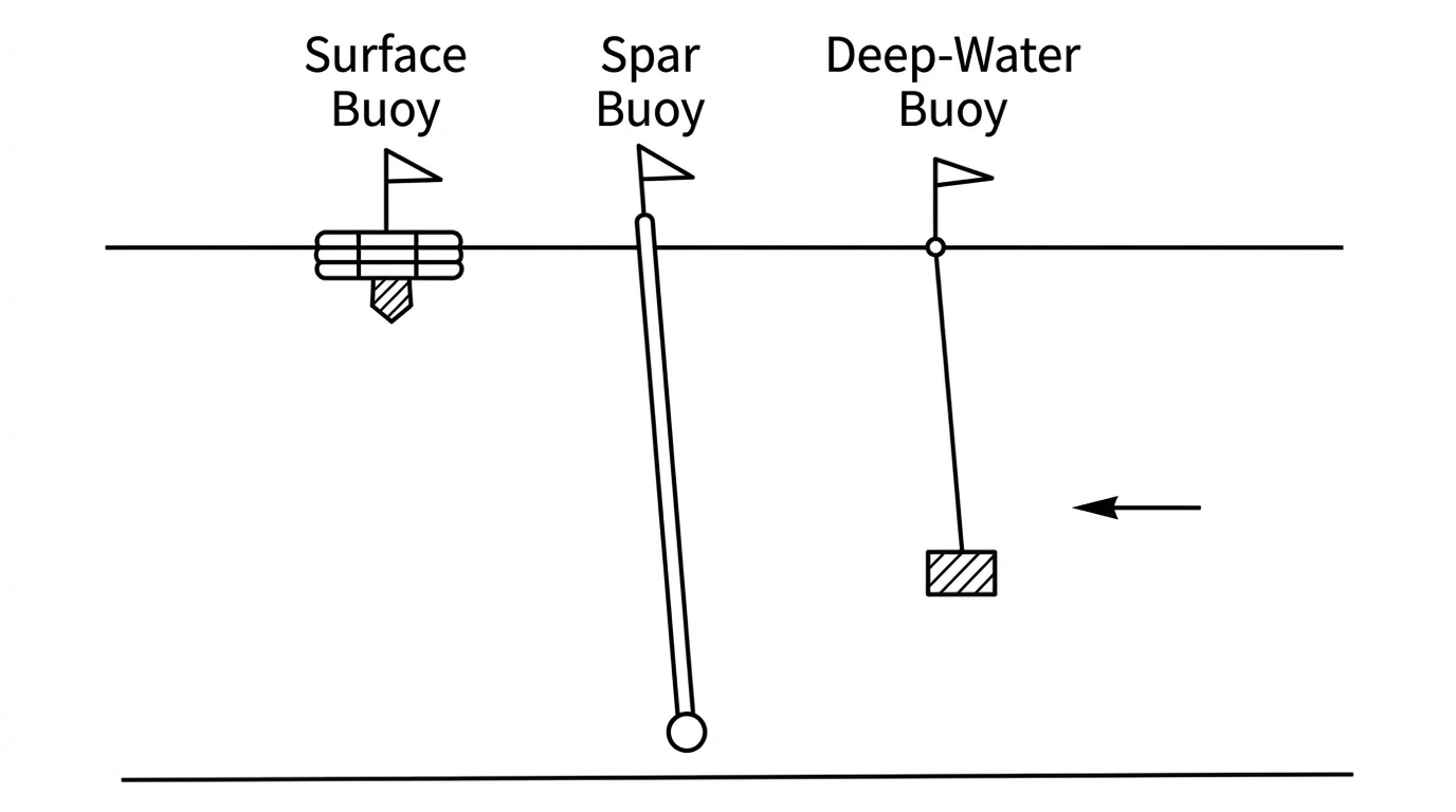
Diagram of three types of buoys
When the float method fails: Once you need numbers that someone else will rely on for money, safety, or legal compliance, the float method becomes a liability. It also fails systematically in deep, slow water where the surface-to-mean ratio breaks down, and in very wide channels where a single float path isn’t representative.
Equipment needed: Float (half-filled water bottle works), stakes, measuring tape, stopwatch. Cost: $0–20.
3.2 Bucket and Stopwatch: Primitive, Perfect
What it is: Divert the entire flow into a container of known volume. Time how long it takes to fill. Divide. Done.
Best for: Tiny flows — springs, siphon tubes, individual sprinkler nozzles, lab calibration setups. Any flow small enough that you can physically catch it all.
Accuracy reality: ±1–3% if done carefully. This is the reference standard against which other methods are sometimes calibrated.
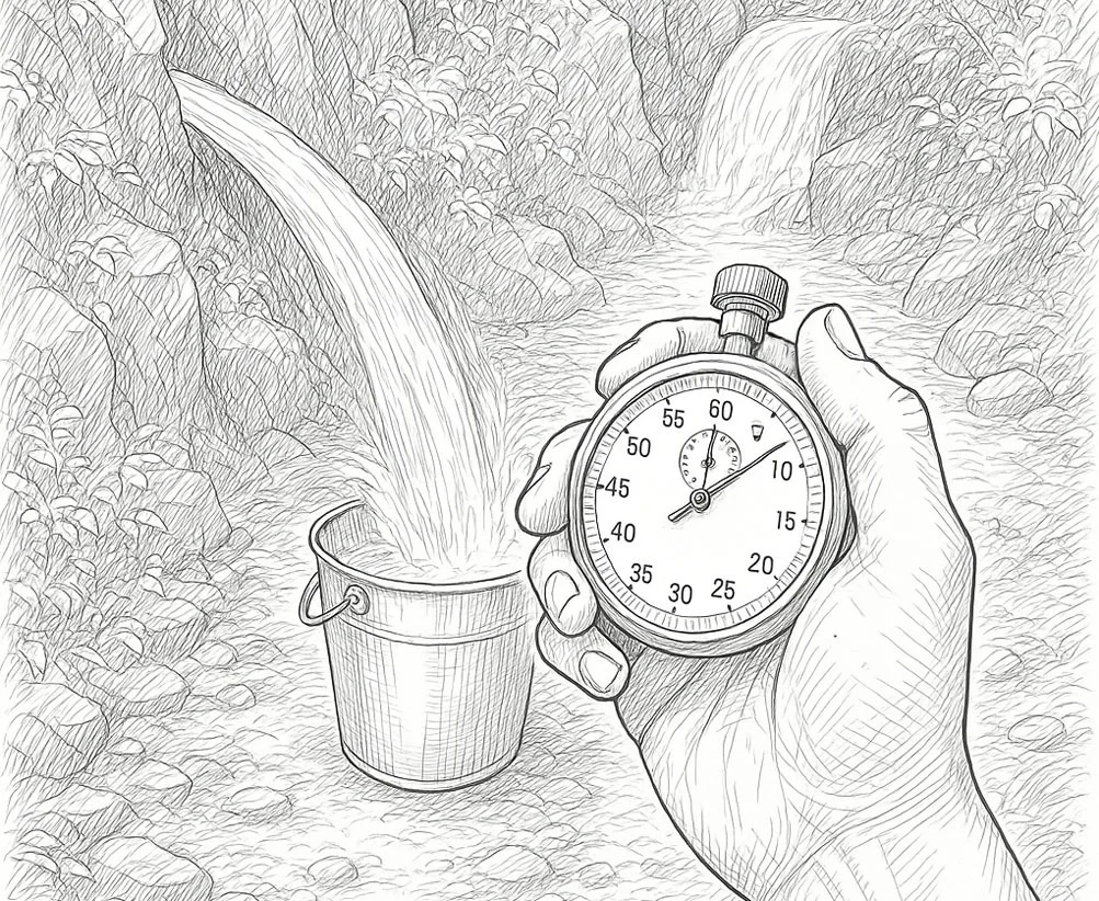
bucket method
When the bucket method fails: The moment the flow exceeds what you can physically capture. Also: this method measures a sample in time, not continuous flow. If the source fluctuates, take multiple measurements and average.
Equipment needed: Bucket or graduated container, stopwatch, pipe or dam to divert flow. Cost: $10–50.
3.3 Mechanical Current Meter: The 20th-Century Workhorse
What it is: A propeller or cup wheel immersed in the flow. Rotations per second map to velocity via a calibration equation. You divide the channel into vertical subsections, measure velocity at 0.6 depth (or average of 0.2 and 0.8 depth for deeper water), multiply by subsection area, and sum.
Best for: Rivers and canals where ±5% is good enough, budgets are moderate, and you don’t need real-time data. This is still how most national hydrological services (USGS included) perform their manual discharge measurements.
Accuracy reality: ±2–5% when performed by a trained hydrographer following standard protocols (ISO 748, USGS techniques). The operator matters as much as the instrument.
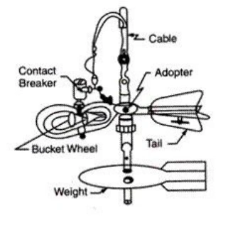
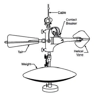
Price current-meter(left) & Amsler current-meter(right)
When the current meter fails: High sediment loads wear down bearings. Weed and debris foul the propeller. Very low velocities (<0.05 m/s) won’t spin the rotor reliably. And it’s labor-intensive — a full discharge measurement on a medium river takes 30–90 minutes, during which flow must remain steady.
Equipment needed: Current meter (propeller or cup type), wading rod or suspension cable, revolution counter, survey tape. Cost: $1,500–5,000.
3.4 Weirs: Turn Flow Into Height, Then Do Math
What it is: A precisely shaped barrier across the channel with a notch (V-shaped or rectangular). Water backs up and spills over. The depth of water above the crest — called head — has a known physical relationship to flow rate. Measure the head, calculate the flow.
Best for: Small to medium channels where you can afford the head loss, need continuous recording, and want something mechanical with no moving parts. Agricultural runoff monitoring, small wastewater treatment outfalls, research watersheds.
V-notch (triangular) weir: Best for highly variable flows, small discharges (<114 L/s). High accuracy at low flows because small changes in head produce measurable changes in the V cross-section.
Rectangular weir: Best for larger, steadier flows. Requires more careful construction and a longer approach channel.
Accuracy reality: ±3–5% when built and maintained correctly. Accuracy degrades when the weir crest wears, when sediment fills the upstream pool, or when the downstream water level rises high enough to submerge the nappe (the free-falling sheet of water).
When weirs fail: They need free-fall conditions — adequate drop downstream. They trap sediment upstream. They back up water, which can flood upstream land or infrastructure. And they are a physical obstruction in the channel that fish, debris, and boats cannot pass.
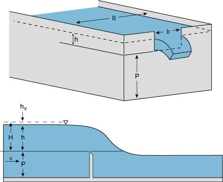
Complete sectional structural diagram of a rectangular thin-walled weir
Equipment needed: Construction materials (wood, sheet metal, concrete), level sensor (ultrasonic/radar/float) for continuous recording, staff gauge. Construction cost: $500–5,000+ depending on materials and channel size.
3.5 Flumes: The Low-Head Alternative
What it is: A specially shaped channel constriction that accelerates flow to critical velocity, creating a predictable relationship between water depth and discharge. Parshall flumes are the most widely standardized.
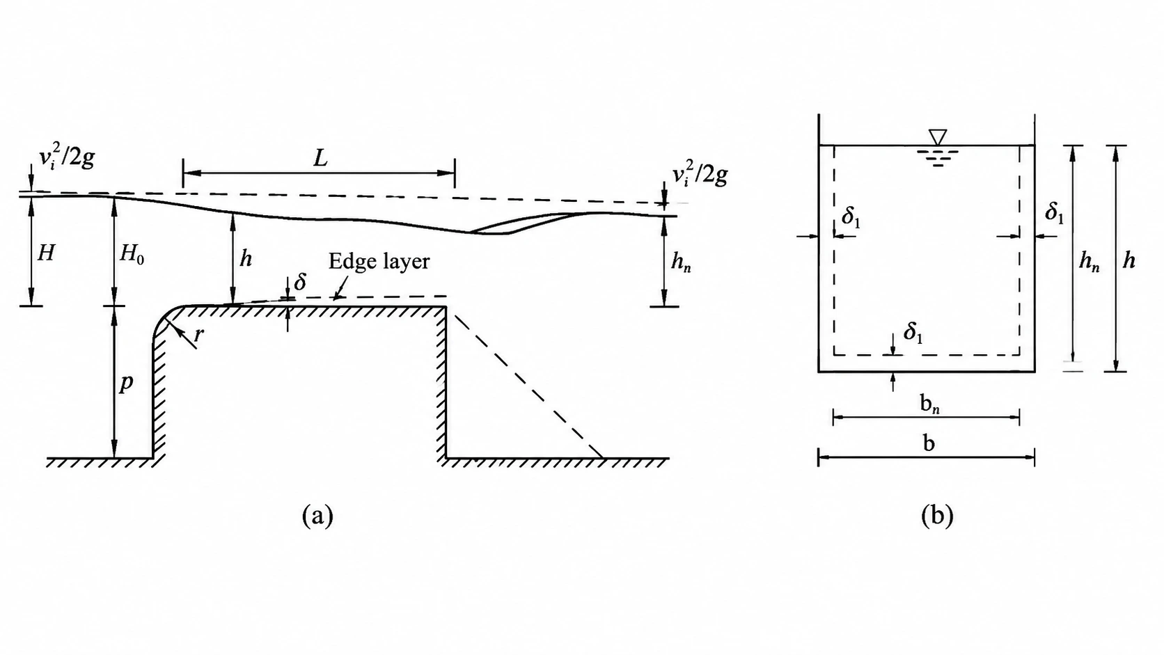
Longitudinal Section Diagram of Riverbed-style Trough
Best for: Canals and channels where you cannot tolerate the head loss a weir requires. Wastewater treatment plants (Palmer-Bowlus flumes for partially filled pipes). Irrigation districts. Situations with sediment or debris that would accumulate behind a weir.
Accuracy reality: ±3–5% for Parshall flumes under standard conditions. Cutthroat flumes are slightly less accurate but cheaper to build.
When flumes fail: Submergence — when the downstream water backs up into the flume — destroys the critical flow assumption and invalidates the rating. Flumes also require precise dimensional construction; a few centimeters of error in the throat width can throw off flow calculations significantly.
Equipment needed: Prefabricated flume or in-situ concrete construction, upstream level sensor. Cost: $1,000–15,000.
Open Channel Methods: Quick Comparison
| Method | Flow Range | Typical Accuracy | Labor Intensity | Continuous? | Relative Cost |
|---|---|---|---|---|---|
| Float | 0.1 – 50 m³/s | ±20–40% | Low | No | Minimal |
| Bucket | 0.001 – 0.005 m³/s | ±1–3% | Low | No | Minimal |
| Current meter | 0.01 – 1,000 m³/s | ±2–5% | High | No | Moderate |
| V-notch weir | 0.0001 – 0.1 m³/s | ±3–5% | Low (after installation) | Yes | Moderate |
| Rectangular weir | 0.01 – 10 m³/s | ±3–5% | Low (after installation) | Yes | Moderate |
| Parshall flume | 0.01 – 50 m³/s | ±3–5% | Low | Yes | Higher |
4. Closed Pipe Methods: When Water Travels Under Pressure
Pipes are deceptively familiar. The water is contained, the geometry is cylindrical — shouldn’t this be easier than open channels? In some ways, yes. In one crucial way, no: you can’t see inside the pipe. Every pipe flow measurement relies on inference from indirect signals, and every inference can be fooled.
4.1 Electromagnetic Flow Meters (Magmeters): The Industry Standard
What it is: Faraday’s law in action. A magnetic field is generated across the pipe. Conductive water flowing through it induces a voltage proportional to velocity. No moving parts, nothing protruding into the flow.
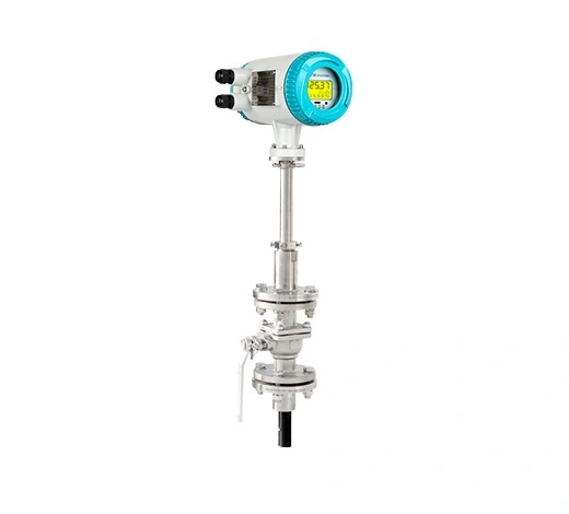
Insertion Electromagnetic Flowmeter
Best for: Water and wastewater treatment plants. Any application with conductive fluid (>5 µS/cm — tap water, river water, wastewater all qualify). Sludge, slurries, and chemically dosed water. Custody transfer where ±0.5% accuracy is required and the budget can support it.
Accuracy reality: ±0.2–0.5% of rate — among the best of any flow technology. Accuracy is stable over years with proper installation.
When magmeters fail: The fluid must be conductive. Deionized water, ultrapure water, and most hydrocarbons won’t work. The pipe must run full at all times. Air bubbles passing through the meter create massive spikes. And magmeters are sensitive to electrical noise — don’t install one next to a variable-frequency drive without proper grounding.
Installation minimums: 5× pipe diameter straight run upstream, 3× downstream. Full-pipe condition mandatory.
Cost: $2,000–15,000 depending on size, liner material, and certification requirements.
4.2 Ultrasonic Flow Meters: Clamp It On and Go
Transit-time principle: Two transducers send ultrasonic pulses diagonally across the pipe — one upstream, one downstream. The downstream pulse travels slightly faster (carried by the flow), and the time difference reveals the average velocity along the acoustic path.
Doppler principle: Sound reflects off particles or bubbles in the fluid. The frequency shift of the returned signal is proportional to velocity. Requires some suspended material in the water.
Best for: Transit-time: clean water, large pipes, permanent installations where you want no pressure loss. Doppler: dirty water, wastewater, slurries. Clamp-on versions: retrofit situations where cutting into the pipe is impossible or prohibitively expensive.
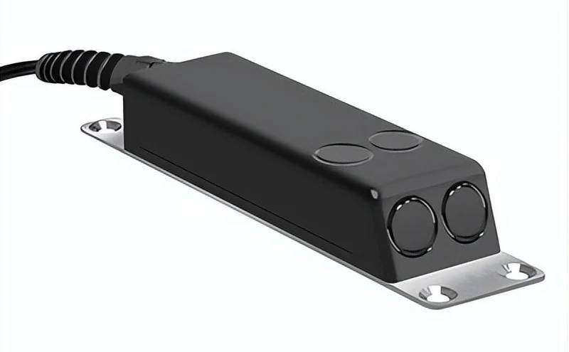
Diving Doppler ultrasound probe (river open channel submerged, commonly used in hydrology)
Accuracy reality: Transit-time: ±1–2%. Doppler: ±2–5%. Clamp-on installation reduces accuracy slightly vs. inline (wetted) transducers.
When ultrasonic fails: Transit-time requires a clean acoustic path — heavy sediment, gas bubbles, or pipe wall scaling degrade the signal. Doppler needs enough particles to reflect off; crystal-clear mountain streams might give a weak return. Both are sensitive to pipe material — concrete, lined pipe, and some plastics attenuate ultrasound.
Unique advantage: Clamp-on ultrasonic is the only technology that lets you measure flow in an existing, operating pipe without any cutting, welding, or process interruption. For temporary surveys, leak detection campaigns, or verification of existing meters, this is transformative.
Cost: $3,000–20,000 (clamp-on portable units at the low end, inline multi-path systems at the high end).
4.3 Turbine and Propeller Meters: Simple Mechanics
What it is: A rotating element spins at a rate proportional to flow velocity. Count the rotations. Mechanical totalizers or magnetic pickups convert to flow rate and totalized volume.
Best for: Clean water in irrigation pipelines, well discharge monitoring, district water supply metering. Anything where moderate accuracy (±1–2%) at moderate cost is the target.
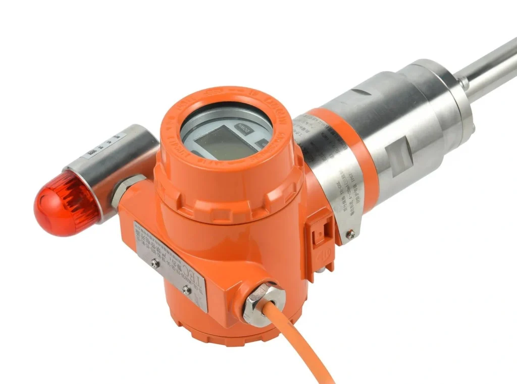
Integrated Pipeline Turbine Flowmeter(left) & Propeller Flowmeter with Handheld Readout(right)
Accuracy reality: ±1–2% within the specified flow range. Accuracy degrades at the low end of the range (bearing friction becomes significant relative to flow force). Degrades over time as bearings wear.
When turbine meters fail: Dirt, debris, or scaling on the rotor. Low flows. Pulsating flow from piston pumps. Installation too close to valves or elbows. These meters have moving parts in the flow stream — everything that can wear, will wear.
Maintenance reality: Plan on bearing replacement and recalibration every 2–4 years depending on water quality and operating hours. This is a real lifecycle cost that users of “cheaper” mechanical meters often fail to budget for.
Cost: $500–5,000 for typical sizes.
4.4 Differential Pressure (DP): The Old Guard
What it is: Insert a restriction — orifice plate, Venturi tube, flow nozzle, V-cone — into the pipe. Measure the pressure drop across it. Flow rate is proportional to the square root of that pressure difference. This is the most mature flow measurement technology, backed by a century of standards (ISO 5167).
Best for: High-temperature, high-pressure applications where electronic meters can’t survive. Steam. Large-diameter pipes where custom fabrication is more economical than a full-bore magmeter. Environments where traceable, standards-based measurement is required and you’re willing to sacrifice energy efficiency for it.
Accuracy reality: ±1–2% of full scale for a well-installed orifice plate with proper tapping and a good differential pressure transmitter.
The hidden cost: Permanent pressure loss. An orifice plate typically wastes 40–80% of the measured differential pressure as unrecoverable head loss. In a large pumping system, this translates directly to higher electricity bills — year after year. Venturi tubes recover more pressure but cost more to fabricate.
When DP fails: Wear on the orifice plate edge changes the discharge coefficient. Improper tap location. Pulsating flow. Two-phase flow (water + air). Low Reynolds numbers where the discharge coefficient is no longer constant.
Cost: $1,000–10,000+ (orifice and transmitter at the low end, custom Venturi at the high end).
Closed Pipe Methods: Quick Comparison
| Method | Accuracy | Pressure Loss | Moving Parts | Straight Pipe Needed | Maintenance Burden | Relative Cost |
|---|---|---|---|---|---|---|
| Magnetic | ±0.2–0.5% | None | None | 5D up / 3D down | Very low | $$$ |
| Ultrasonic (Transit-time) | ±1–2% | None | None | 10D up / 5D down | Low | $$$ |
| Turbine | ±1–2% | Low | Yes (bearings) | 10D up / 5D down | Moderate (recalibration) | $$ |
| Orifice plate (DP) | ±1–2% FS | High (40–80%) | None | 10–30D up / 5D down | Moderate (plate inspection) | $$ |
| Venturi (DP) | ±1% | Low–Moderate | None | 10–30D up / 5D down | Low | $$$ |
5. The Accuracy Trap: Why ±1% Doesn’t Mean What You Think
A spec sheet says “Accuracy: ±0.5% of reading.” You install the meter. You get a number. You report it with confidence.
Here’s what actually happened, in a real project we consulted on: a ±0.5% electromagnetic flow meter was installed three pipe diameters downstream of a 90° elbow. Swirling, asymmetric flow entered the meter. The actual error was approximately 15%. The meter was fine. The installation was the problem.
And the client — a water utility that relied on these numbers for billing — had been systematically undermeasuring for two years.
The Accuracy Chain
Instrument accuracy is the first link in a chain, not the last. The true accuracy of your measurement is determined by the weakest link in this chain:
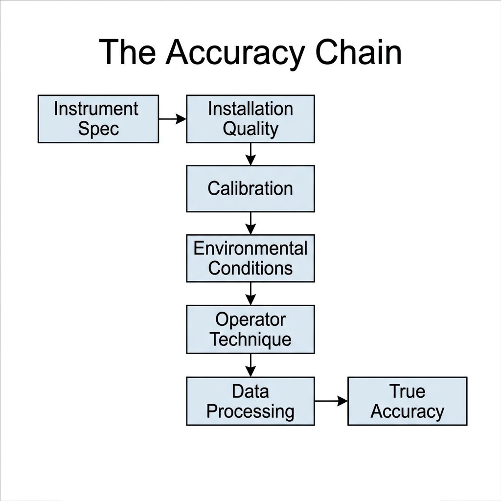
A ±0.2% Coriolis meter with a bad installation might produce ±5% data. A ±5% current meter handled by an experienced hydrographer following ISO 748 procedures might give you ±2%.
Concrete example: The USGS standard for streamflow measurement using a mechanical current meter is ±5% under ideal conditions. But USGS field protocols specify minimum numbers of verticals (25–30), specific depth-measurement methods, and maximum allowable velocity variation between subsections. Follow the standard and you get ±5%. Skip half the verticals because you’re in a hurry, and your “±5% instrument” is now giving you ±15%.
What Accuracy Do You Actually Need?
This is the question that distinguishes good measurement from wasted money. Here’s a practical guide:
| Application | Required Accuracy | Why |
|---|---|---|
| Flood early warning | ±15–20% | You need to know the water is rising fast — the trend matters more than the absolute number |
| Irrigation scheduling | ±10% | Crops are forgiving; pumping cost optimization is the real driver |
| Environmental flow monitoring | ±5–10% | Ecological thresholds need reasonable precision |
| Water rights / inter-district allocation | ±2–5% | Money and legal agreements depend on these numbers |
| Scientific research | ±0.5–2% | Peer review demands defensible uncertainty estimates |
| Custody transfer / billing | ±0.5% or better | Every percentage point is revenue |
The lesson: Before you look at instruments, define your minimum acceptable accuracy. Then work the accuracy chain backward: what installation, calibration, and operational practices are required to protect that number? If you can’t meet those requirements with a given instrument, no amount of spending on a higher-spec sensor will help.
Key Insight: The most expensive meter is not the one with the highest price tag. It’s the one that gives you wrong numbers that someone acted on.
6. ADCP: The Method That Changed the Game
Everything we’ve discussed so far — current meters, weirs, flumes, magmeters — shares one fundamental limitation: they measure velocity at a point (or infer an average from a single path) and then extrapolate to the whole cross-section.
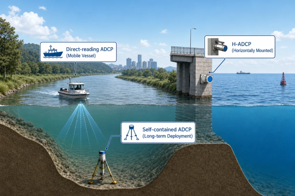
An Acoustic Doppler Current Profiler (ADCP) doesn’t do that. It measures velocity simultaneously at hundreds of points across the entire water column, building a complete velocity profile in three dimensions.
What Makes ADCP Fundamentally Different
A traditional current meter gives you this: one number, at one depth, at one horizontal position. To get a full discharge measurement, you have to take 20–30 individual measurements across the channel, each at one or two depths, and integrate. A skilled team on a medium river takes 30–90 minutes.
An ADCP mounted on a small boat (or a remote-controlled USV) moving across the same river gives you the entire velocity cross-section — surface to bed, bank to bank — in a single transect lasting 3–5 minutes. Instead of 30 data points, you have thousands. Instead of assuming the velocity profile follows a theoretical curve, you measure it directly.
The paradigm shift isn’t “better accuracy” (though ADCP accuracy is excellent at ±0.5–2%). The paradigm shift is data density. You’re no longer estimating the flow — you’re directly observing the velocity field.
Where ADCP Excels
- Large rivers (Amazon, Congo, Yangtze scale): Where traditional current-meter measurements take a full day and still miss complex secondary currents, ADCP completes the job in under an hour with superior spatial resolution.
- Tidal and estuarine environments: Bidirectional flow that reverses every six hours is nearly impossible to capture with single-point methods. ADCP profiles continuously through the tidal cycle.
- Deep ocean: Mooring-mounted ADCPs profile currents from the seafloor to the surface for months or years — data that is essential for offshore engineering, climate research, and navigation safety.
- Complex velocity fields: Braided rivers, confluence zones, behind bridge piers — anywhere the flow isn’t simple, single-point methods break down and profiling methods shine.
When ADCP Is Not the Right Choice
Transparency matters. ADCP is not the universal answer:
- Very shallow water (<0.3 m): The acoustic beams need a minimum depth to measure. Below 0.3 meters, the instrument’s blanking distance and side-lobe interference make ADCP unreliable. A weir or flume is better.
- Budget-constrained spot measurements: If you’re checking an irrigation turnout once a month and ±10% is fine, a $500 propeller meter plus wading rod is the rational choice — not a $20,000 ADCP system.
- Clean-water pipes under 12 inches: A clamp-on ultrasonic flow meter ($3,000–8,000) will match ADCP accuracy for pipe flow at a fraction of the cost. ADCP is designed for open water, not pressurized pipes.
- Permanent single-point monitoring: If you only need to know “is the water rising above alarm level?”, a simple radar level sensor with a rating curve is more cost-effective than an ADCP station.
The right question is never “should I buy an ADCP?” It’s “what kind of water am I measuring, what decisions depend on the data, and which tool maps most directly to those requirements?”
Recommended reading: For a deeper dive into ADCP technology, see our articles on the ADCP Working Principle, Frequency Selection Guide, and ADCP vs. Traditional Current Meters.
For river-specific applications, refer to our ADCP for River Flow Measurement guide and ADCP Applications in River Discharge Measurement.
7. Your Decision Framework: From “What Should I Use?” to “I Know What to Buy”
Here’s the decision path that integrates everything we’ve covered. Start at the top.
Decision Tree: Water Flow Measurement Method Selection
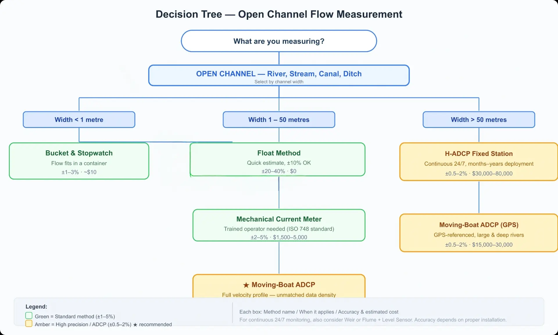
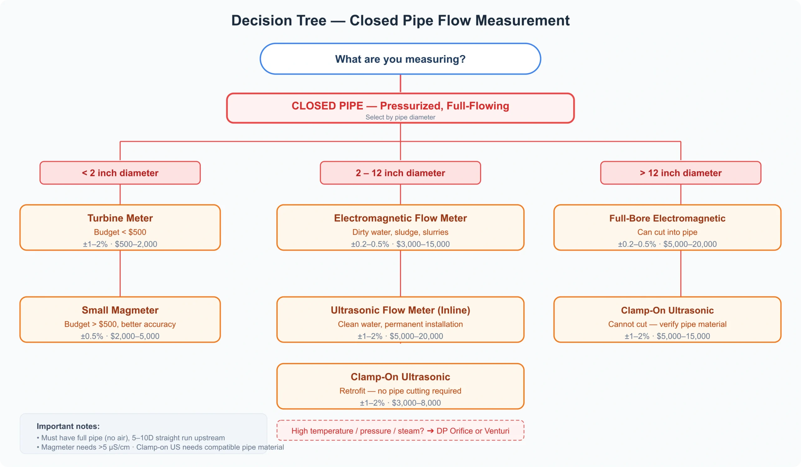
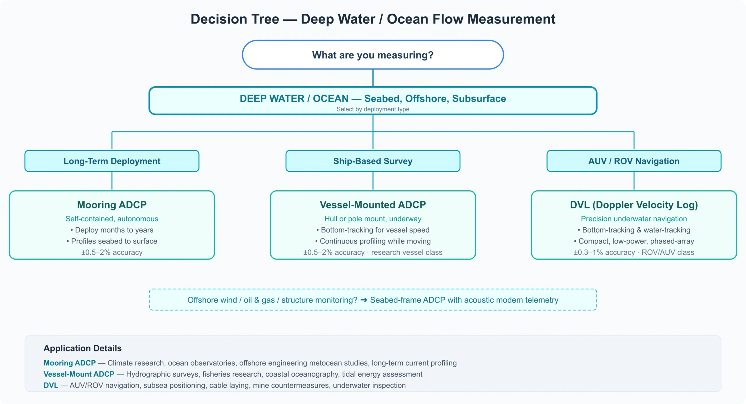
For an interactive tool that walks you through ADCP model selection specifically, contact Oceantek engineering team
The 5-Question Reality Check
Before you commit to any method, answer these five questions honestly:
- Who will install it? If the answer is “Bob from maintenance,” pick the method with the most forgiving installation requirements. A magmeter with insufficient straight pipe is worse than a turbine meter installed correctly.
- Who will maintain it? A weir needs sediment clearing. A turbine meter needs bearing replacement. An ADCP needs firmware updates and occasional recalibration. No instrument is zero-maintenance — but some are zero-maintenance in your organization’s capabilities.
- What happens if the number is wrong? If the consequence is “someone writes an angry email,” your tolerance is higher than if “the EPA fines us $50,000.” Define the cost of error before you define the budget for accuracy.
- Will conditions change over the life of the installation? A riverbed scours and fills. A pipe scales and corrodes. A weir pool silts in. If your measurement method can’t handle the range of conditions it will actually encounter, it’s the wrong method.
- Can you validate the measurement independently? Every installation should include a plan for occasional verification — a redundant measurement, a tracer dilution test, a bucket check. If there’s no way to check the meter, you’re flying blind.
8. The Future of Water Flow Measurement
The technology is moving fast in three directions:
Direction 1: From single-point to profiling. The shift from current meters to ADCP in open channels isn’t complete, but the trend is clear. The next frontier is phased-array ADCP with electronic beam steering — eliminating the moving parts of mechanical beam assemblies while retaining full profiling capability. See our article on phased-array ADCP technology.
Direction 2: From manual to autonomous. Unmanned surface vessels (USVs) carrying ADCP are replacing manned boats for river discharge measurement — reducing labor, improving safety, and enabling measurements during flood conditions when manned surveys are impossible. Read more about USV ADCP operations.
Direction 3: From data to decisions. The raw flow number is becoming the input to AI-powered systems that integrate it with weather forecasts, soil moisture, and operational schedules to make automated decisions — opening dam gates, adjusting pump speeds, issuing flood warnings. The instrument is no longer the product; the decision is.
9. Quick Reference: Standards and Formulas
Key Formulas
| Formula | Use |
|---|---|
| Q = A × V | Fundamental flow equation: Discharge = Cross-sectional area × Mean velocity |
| Q = 2.49 × H2.48 | 90° V-notch weir (Q in cfs, H in feet) |
| Q = 3.33 × (L − 0.2H) × H1.5 | Rectangular weir (contracted) |
| Manning equation | Open-channel velocity from channel roughness, slope, and hydraulic radius |
Relevant Standards
| Standard | Scope |
|---|---|
| ISO 748 | Flow measurement in open channels — velocity-area methods |
| ISO 5167 | Flow measurement with differential pressure devices in full pipes |
| ISO 2425 | Measurement of flow in tidal channels |
| ASTM D5640 | Standard guide for selection of weirs and flumes |
| USGS TWRI Book 3, Ch. A8–A22 | USGS streamgaging techniques and standards |
| AWWA M33 | Flowmeters in water supply |
10. Frequently Asked Questions
For small flows: the bucket-and-stopwatch method (volumetric) is the gold standard at ±1%. For larger open channels: an ADCP operated according to ISO 748 procedures achieves ±0.5–2%. For pressurized pipes: a properly installed Coriolis meter achieves ±0.1–0.5%. But remember — installation quality often matters more than the instrument’s rated accuracy.
The float method is the fastest zero-equipment approach: time a floating object over a known distance, estimate the channel cross-section, multiply surface velocity × cross-section area × 0.85 (correction factor). Expect ±20–40% accuracy. Better than nothing, but not suitable for any situation involving money, safety, or regulatory compliance.
Velocity is speed (m/s). Flow rate is volume per time (m³/s, L/s, GPM, cfs). Flow rate = Mean velocity × Cross-sectional area. The distinction matters because you can have high velocity in a small pipe (low flow rate) or low velocity in a wide river (enormous flow rate).
Manufacturers typically recommend annual calibration for critical applications, every 2–3 years for general use. Mechanical meters (turbine, propeller) need more frequent recalibration as bearings wear. Electromagnetic and ultrasonic meters are more stable but should still be verified periodically against a reference measurement. In practice, many organizations calibrate far less often than they should.
Generally no. A float method that works tolerably for a 5-meter-wide stream becomes nearly meaningless on a 500-meter-wide river where velocity varies dramatically across the channel. Conversely, an ADCP that’s perfect for the Amazon would be physically impractical in a 30-cm-wide irrigation ditch. Method selection is fundamentally about matching the tool to the scale.
The top five error sources, in rough order of frequency: (1) inadequate straight pipe/channel run upstream, (2) air entrainment or non-full-pipe conditions, (3) incorrect velocity-to-mean-velocity conversion, (4) poor cross-sectional area measurement, (5) instrument calibration drift or damage. Notice that only one of the top five is about the instrument itself.
A rating curve (stage-discharge relationship) correlates water level to flow rate for a specific location. If you’re doing continuous monitoring of a river or open channel, you almost certainly need one — water level is cheap to measure continuously; direct flow measurement is not. The rating curve is developed from periodic discharge measurements (using current meter or ADCP) across a range of flow conditions, then used to convert the continuous level record into continuous flow data.
An ADCP is a type of flow measurement instrument, but the term “flow meter” usually refers to pipe-flow devices (electromagnetic, ultrasonic, turbine meters installed inline in pressurized pipes). ADCP is designed for open water — rivers, oceans, canals — and measures velocity profiles rather than a single averaged velocity. They serve different applications, and choosing between them is about where the water is, not which technology is “better.”
Most ADCPs require approximately 0.3–0.5 meters minimum depth, depending on frequency and transducer configuration. Below this, the acoustic beams don’t have enough range to profile meaningfully, and the instrument’s blanking distance becomes a significant fraction of the total depth. For very shallow water, a weir, flume, or current meter is more appropriate.
The range is extreme. A float test costs nothing. A mechanical current meter costs $1,500–5,000. A portable ADCP system costs $15,000–30,000. A permanent horizontal ADCP monitoring station can run $30,000–80,000 installed. A full-bore electromagnetic meter for a large municipal pipe is $5,000–15,000. The question isn’t “how much does it cost?” but “what does getting the number wrong cost?”
11. Ready to Choose an Instrument? Explore Our Product Lines
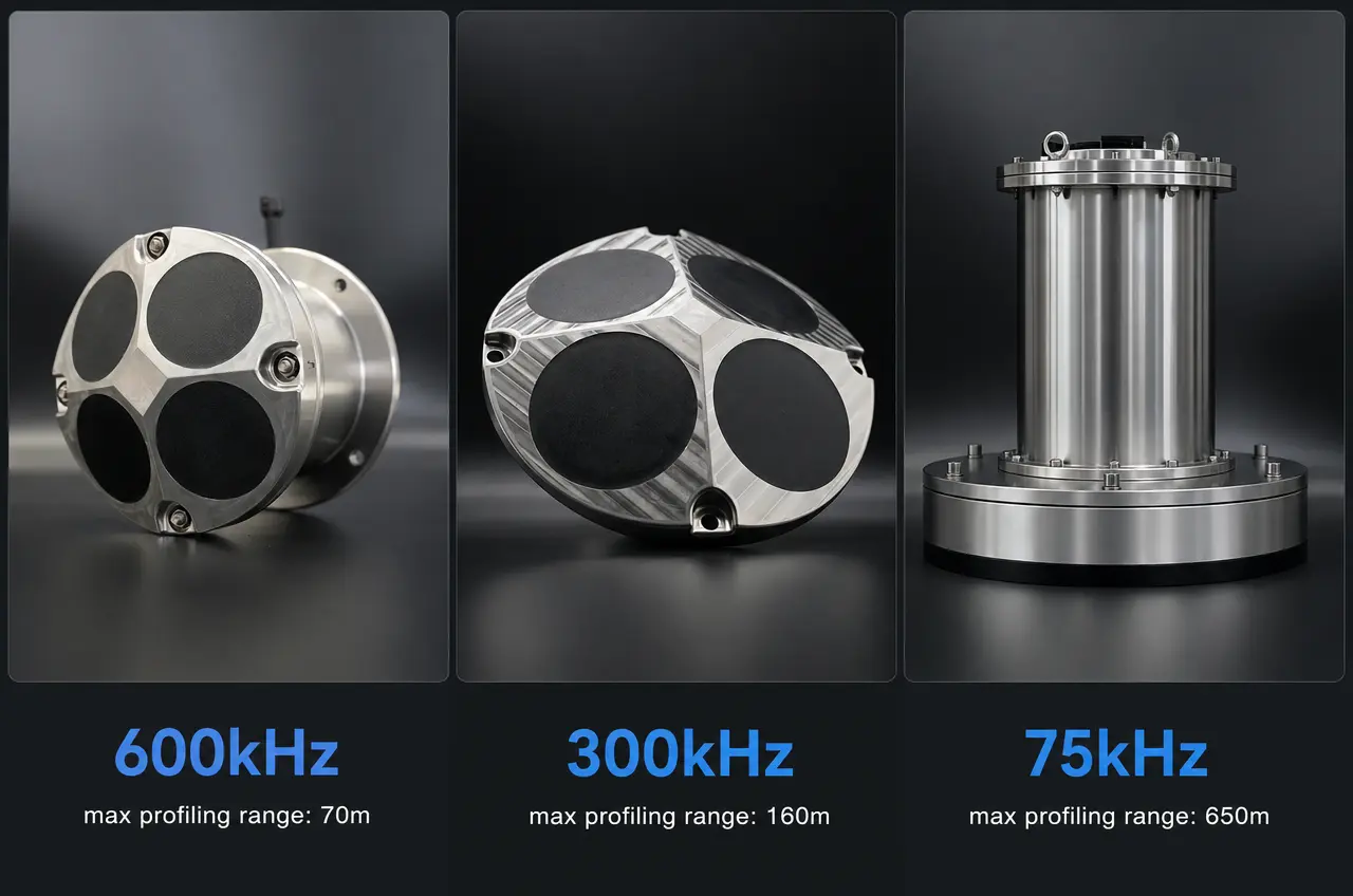
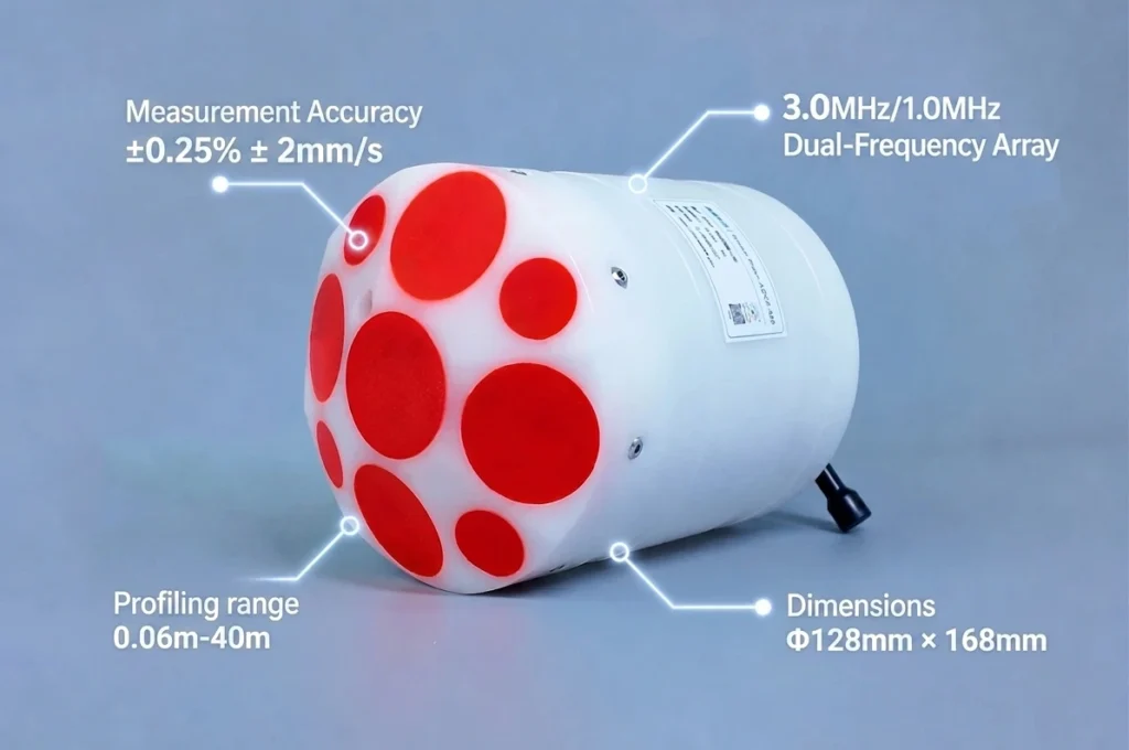
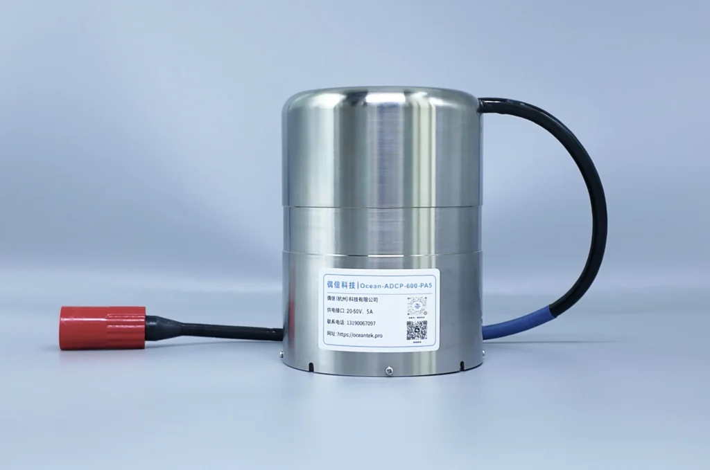
This guide covered the full landscape of water flow measurement methods — from a $10 bucket to a $80,000 ADCP monitoring station. If your decision tree pointed you toward ADCP or DVL technology, here are the Oceantek product families that match each scenario:
| Your Application | Recommended Product Line | Key Models |
|---|---|---|
| River discharge — portable, quick surveys Wading or boat-mounted, one transect in 3–5 minutes | River ADCP Series | River ADCP M9 (9-beam), H-ADCP 600 |
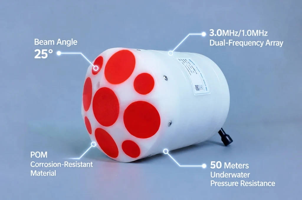
| River / canal / coastal — fixed installation Tripod, bridge pier, or bottom mount; real-time data via cable | Direct-Reading ADCP Series | ADCP-300-DR-FA4, ADCP-600-DR-FA4, ADCP-75-DR-PA4, OCEAN-ADCP-600-PA5 |
| Deep ocean — long-term autonomous deployment Mooring-mounted, months to years, seabed-to-surface profiling | Self-Contained ADCP Series | ADCP-300-SC-FA4, ADCP-600-SC-FA4, ADCP-75-SC-PA4 |
| AUV / ROV — underwater navigation Bottom-tracking and water-tracking, compact phased-array | DVL Series | DVL-300-DR-FA4, DVL-600-DR-FA4, DVL-600-DR-PA5 |
| Quick spot checks — shallow water Single-point velocity, handheld or rod-mounted | Single-Point Current Meter | Portable point velocity sensor |
| Underwater acoustics — listen or track Passive acoustic monitoring, positioning reference | Self-Contained Hydrophone | Autonomous acoustic recorder |
For side-by-side comparisons with other brands, see our 2026 ADCP Brand Comparison. For real-world validation, browse 20+ river case studies — from the Amazon to the Yangtze — in our Case Studies Library.
Last updated: July 2026. This guide is maintained by the Oceantek technical team. For specific application questions or instrument selection support, visit our contact page.