Author’s Note: This article draws on peer-reviewed oceanographic research, operational data from maritime safety agencies, and direct technical consultation with ocean instrumentation engineers. All technology specifications are verifiable against published manufacturer data sheets and academic literature.
Introduction
In September 2024, a container ship navigating the East China Sea encountered an unexpected surface current that pushed it 2.3 nautical miles off course in under an hour. The deviation was caught — not by GPS alone, but by a network of ocean profiling instruments that had mapped the current field days earlier. The ship’s routing software, fed with profile data, had already flagged the area. The crew adjusted course. A near-miss became a non-event.
Ocean profiling is the quiet infrastructure behind much of what we know — and need to know — about the sea. It underpins climate models that forecast monsoon intensity. It guides search-and-rescue teams deciding where to deploy. It tells offshore engineers whether conditions are safe to lower a 200-ton subsea structure to the seabed.
Yet outside specialist circles, it is poorly understood.
In this article, we’ll examine:
- What ocean profiling actually measures — and why those parameters matter
- How profiling data serves marine research across climate science, ecosystem monitoring, and fisheries management
- How it protects human life at sea — from search-and-rescue drift prediction to offshore operational safety
- The instruments that collect profile data, how they work, and how to choose the right tool
- Concrete case studies where profiling data made the difference
1. What Is Ocean Profiling?
The Basic Concept
Ocean profiling is the measurement of physical, chemical, and biological parameters of seawater as a function of depth. Instead of a single reading at the surface, a profile is a vertical column of data — a high-resolution picture of how conditions change from the air-sea interface down to the seabed.
Think of it as the difference between a single photograph and a CT scan. The photograph (a surface measurement) tells you what’s happening at one slice. The CT scan (a profile) reveals the full three-dimensional structure.
What Parameters Does Ocean Profiling Measure?
| Parameter | What It Tells Us | Why It Matters |
|---|---|---|
| Current velocity & direction | How water moves at each depth layer | Navigation safety, drift prediction, sediment transport, offshore engineering |
| Temperature | Vertical thermal structure, thermocline depth | Climate monitoring, sonar performance, marine ecosystem health |
| Salinity | Freshwater influence, water mass identification | Ocean circulation models, desalination plant intake planning |
| Depth / Pressure | Precise vertical position of each measurement | Essential for correlating all other parameters by depth |
| Dissolved oxygen | Biological activity, water mass age | Fisheries management, hypoxia monitoring, pollution tracking |
| Turbidity / Backscatter | Suspended particle concentration | Sediment plume monitoring, dredging compliance, visibility estimation |
| Chlorophyll-a (fluorescence) | Phytoplankton biomass | Primary productivity, harmful algal bloom early warning |
| Sound velocity | Acoustic propagation speed through the water column | Sonar calibration, multibeam echosounder correction, submarine detection |
Two Types of Profiling
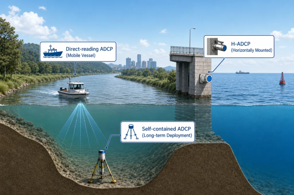
Station-based profiling — An instrument is lowered vertically through the water column from a vessel, mooring, or autonomous platform. It collects a continuous data stream from surface to target depth, then is recovered. Think: a CTD rosette lowered from a research vessel.
Fixed-depth profiling — An instrument mounted at a fixed position (seabed frame, buoy, bridge pier) measures the water column above it using acoustic beams that divide the column into discrete depth cells. Think: an ADCP mounted on the seabed looking upward.
Both approaches are complementary. Station-based profiling gives you a single high-resolution vertical slice at one location and moment. Fixed-depth profiling gives you continuous time-series data — how the profile evolves over hours, days, or seasons — but at a coarser vertical resolution.
2. Ocean Profiling in Marine Research
Marine research depends on ocean profiling the way meteorology depends on weather balloons. Without vertical profiles, oceanographers are working with a flat, two-dimensional view of a fundamentally three-dimensional system.
2.1 Climate Science and Ocean Circulation
The ocean absorbs roughly 90% of the excess heat trapped by greenhouse gases and about 25% of anthropogenic CO₂ emissions. Tracking where that heat and carbon go — how deep, how fast, and along what pathways — is one of the most urgent tasks in climate science.
Ocean profiling makes this possible through:
The Argo Program: An international array of nearly 4,000 autonomous profiling floats that drift with ocean currents, dive to 2,000 meters every 10 days, and ascend while measuring temperature and salinity. Each float produces a full water-column profile. Argo has fundamentally transformed climate modeling by providing — for the first time — continuous, global, real-time subsurface ocean data.
Research vessel CTD transects: Ships repeat the same survey lines year after year — such as the long-running Line P in the North Pacific or the Atlantic Meridional Transect. These ship-based profiles, collected with CTD rosettes that also capture water samples at discrete depths, provide ground-truth data that calibrates and validates satellite and float measurements.
Key finding from profiling data: The 2024 State of the Climate report, drawing on Argo profiles, confirmed that ocean heat content in the upper 2,000 meters reached a record high for the sixth consecutive year. Without profiling, this trend — and its implications for tropical cyclone intensity, sea level rise, and marine heatwaves — would be invisible.
2.2 Ecosystem Monitoring and Marine Biology
Marine ecosystems are vertically structured. Phytoplankton concentrate near the surface where light penetrates. Zooplankton migrate vertically each day — the largest animal migration on Earth by biomass. Deep-scattering layers of fish and squid hover at midwater depths during daylight, ascending at dusk.
Ocean profiling reveals this vertical architecture:
- Fluorescence profiles map phytoplankton distribution — the base of the marine food web
- Dissolved oxygen profiles identify hypoxic “dead zones” where marine life cannot survive, such as the seasonally expanding zones in the Gulf of Mexico and the Baltic Sea
- Acoustic backscatter profiles from ADCPs detect zooplankton layers and fish schools, providing non-invasive biomass estimates
Practical application — Marine Protected Area (MPA) design: When the government of Palau designed its landmark 500,000 km² marine sanctuary, profiling data on vertical current structure and larval dispersal pathways informed the boundary decisions. Placing a protected area in the wrong current path means larvae drift outside the zone — defeating the purpose of the MPA.
2.3 Fisheries Science and Sustainable Harvest
Commercial fisheries management relies on accurate stock assessment — and stock assessment relies on understanding where fish are. Since many commercially important species (cod, pollock, hake, sardine) occupy specific depth ranges that shift with temperature and oxygen, ocean profiles are a direct input to fisheries models.
Case in point — The Peruvian anchoveta fishery: The world’s largest single-species fishery (4–5 million metric tons annually) depends on the upwelling of cold, nutrient-rich water along the Peruvian coast. Ocean profiling buoys maintained by IMARPE (Instituto del Mar del Perú) continuously monitor thermocline depth and upwelling intensity. When the thermocline deepens beyond a threshold — a sign of El Niño conditions — catch quotas are adjusted before the fleet sails. The alternative — discovering the anchoveta have dispersed after the fleet returns empty — is economically devastating.
2.4 Geological Oceanography and Seabed Mapping
Ocean profiling does not only look upward from the seabed — it also looks downward toward it. Multibeam echosounders and sub-bottom profilers map seafloor bathymetry and sediment layers, supporting:
- Tsunami hazard modeling — tsunami wave propagation depends on seafloor topography
- Submarine landslide risk assessment — sediment instability on continental slopes can trigger tsunamis
- Offshore infrastructure siting — wind farms, cables, and pipelines require detailed seabed characterization
Current profile data is equally important for geological work: sediment transport models that predict coastal erosion and sandbank migration depend on measured near-bed current velocities — data that only ocean profiling instruments can provide.
3. Ocean Profiling in Maritime Safety
If marine research is the “why” of ocean profiling, maritime safety is the “so what.” Profiling data saves lives — directly and measurably.
3.1 Search and Rescue (SAR) Drift Prediction
When a person falls overboard, a fishing vessel goes missing, or an aircraft ditches at sea, the search area is not the last known position. It is the area to which wind and currents have carried the target since the incident.
Search-and-rescue authorities use drift models — the U.S. Coast Guard’s SAROPS (Search and Rescue Optimal Planning System) is the most widely emulated — to compute the most probable search area. These models require two inputs: surface wind (from satellites and weather models) and ocean current profiles (from in-situ measurements and ocean circulation models).
Why profiles, not just surface currents? Because a person in the water, a partially submerged vessel, or a life raft each experience different degrees of wind-driven drift versus current-driven drift. A life raft sits high and is pushed primarily by wind. A person in the water is pushed primarily by currents at 0.5–2 meters depth. Drift models must account for the vertical current shear — the difference between surface current and current at the target’s draft depth — to generate an accurate search area.
Measurable impact: The Norwegian Coastal Administration reported that integrating real-time ADCP current profile data from coastal monitoring stations into their drift models reduced the mean search area by 34% compared to wind-only drift prediction. A smaller search area means faster recovery — and in cold water, minutes matter.
3.2 Port Navigation and Vessel Traffic Safety
Large commercial vessels — container ships, tankers, bulk carriers — are increasingly constrained by the margins of modern ports. Approach channels are narrow, under-keel clearance is tight, and cross-currents can push a vessel sideways during the most critical phase of its voyage.
Ocean profiling supports port safety at multiple levels:
Real-time current monitoring at port approaches: Acoustic Doppler current profilers mounted on channel seabeds or bridge piers continuously measure current speed and direction through the full water column. This data is transmitted to vessel traffic services (VTS) and pilots, who use it to:
- Advise inbound vessels on approach timing (slack water vs. peak current)
- Calculate cross-track set during narrow channel transit
- Determine safe under-keel clearance accounting for both tide height and current-induced squat
Historical profile databases for port design: Before a new container terminal is built, engineering consultancies deploy ADCPs for 30–90 days to capture the full spring-neap tidal cycle. The resulting current profile database determines:
- Optimum berth orientation (minimize cross-currents at the berth face)
- Dredging requirements and predicted siltation rates
- Tugboat force requirements for ship handling in worst-case current conditions
3.3 Offshore Energy Operations
The offshore wind industry is on track to install over 380 GW of capacity globally by 2030. Each turbine foundation, each array cable, and each installation vessel depends on accurate current profile data.
During site assessment: Ocean profiling instruments — typically seabed-mounted ADCP frames — are deployed for 30–90 days to characterize the current regime. The data feeds into:
- Foundation design loads (current-induced drag on monopiles and jackets)
- Cable burial depth specification (scour risk assessment)
- Installation vessel operability windows (safe current limits for jack-up vessels and heavy-lift crane barges)
During construction: Real-time current profiles are monitored to ensure that lifting operations stay within safe envelopes. A 2,000-tonne monopile suspended from a crane barge in a 2-knot cross-current is a different engineering problem than the same lift in slack water — and the difference is quantified by profile data.
During operations: Permanent seabed ADCP installations at offshore wind farms provide continuous current monitoring for:
- Crew transfer vessel (CTV) approach safety
- Scour monitoring around foundation bases
- Subsea cable exposure detection after storm events
3.4 Coastal Hazard Early Warning
Storm surge, rip currents, and tsunami waves are all profoundly shaped by the vertical structure of the water column. Ocean profiling provides the subsurface data that makes early warning systems accurate.
Storm surge prediction: Surge height depends on wind stress transferring momentum into the water column — a process governed by vertical mixing, which in turn depends on the density stratification (temperature and salinity profiles). A strongly stratified coastal sea — with a warm, fresh surface layer over cold, saline bottom water — responds differently to wind forcing than a well-mixed water column. Profiling data resolves this ambiguity.
Rip current forecasting: Beach safety agencies in Australia, the United States, and Europe increasingly incorporate nearshore current profile data into rip current risk forecasts. Acoustic profilers deployed in the surf zone measure the vertical structure of rip currents, feeding into models that predict rip intensity based on wave height, tide level, and beach morphology.
Tsunami wave propagation modeling: The speed of a tsunami wave in the open ocean is a function of water depth — specifically, the square root of the product of gravity and depth. Accurate bathymetric profiles along the tsunami’s propagation path are critical for predicting arrival time at distant coastlines. For near-field tsunamis (where the wave arrives within minutes), pre-computed propagation models built on profiling data are the difference between timely evacuation and catastrophe.
4. The Instruments Behind Ocean Profiling
Understanding what ocean profiling achieves requires understanding the tools that make it possible. Here are the four principal instrument categories.
4.1 Acoustic Doppler Current Profilers (ADCPs)
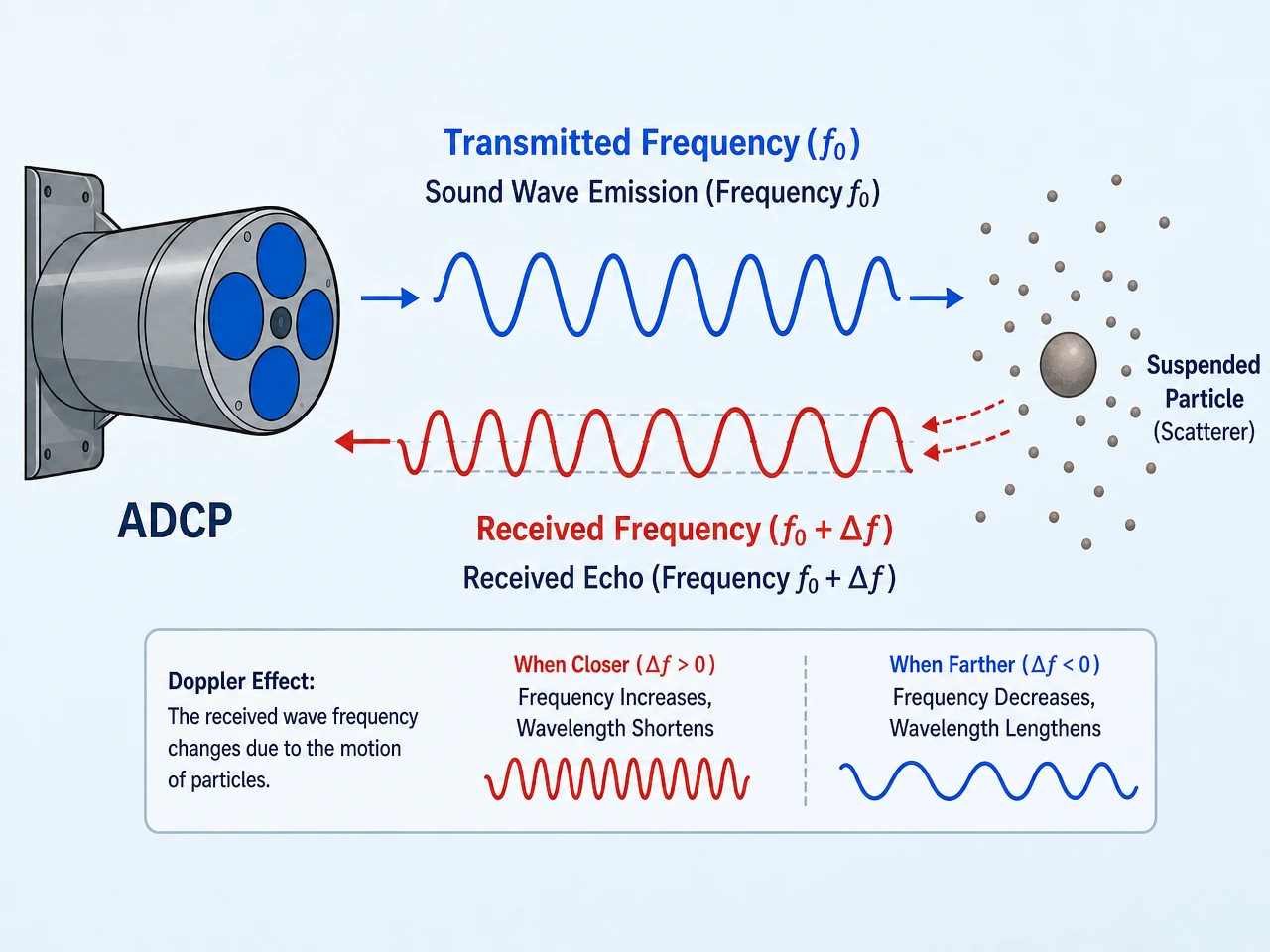
What they measure: Current velocity and direction at multiple depths simultaneously, plus acoustic backscatter intensity.
How they work: An ADCP emits short pulses of sound at a known frequency — typically 75 kHz, 300 kHz, 600 kHz, or 1200 kHz. Suspended particles in the water (sediment, plankton, bubbles) reflect a portion of this sound back to the transducer. The Doppler shift — the change in frequency between the transmitted pulse and the received echo — reveals the speed at which the particles (and therefore the water) are moving toward or away from the instrument.
By dividing the return signal into time-gated “bins,” the ADCP constructs a vertical profile of current velocity. A 600 kHz ADCP with a 1-meter bin size and 50 bins produces a 50-meter current profile — updated every second.
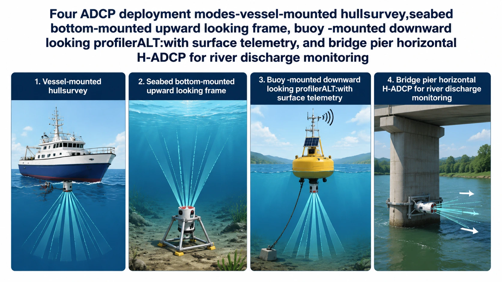
Deployment modes:
| Mode | Description | Typical use |
|---|---|---|
| Vessel-mounted | Transducer fixed to hull or over-the-side pole | Hydrographic survey, river discharge measurement |
| Bottom-mounted (upward-looking) | Frame placed on seabed, transducer facing up | Long-term current monitoring, offshore wind site assessment |
| Buoy-mounted (downward-looking) | Instrument suspended beneath surface buoy | Real-time telemetry to shore, coastal observatories |
| Horizontal (side-looking) | Fixed to bridge pier or channel wall, beam horizontal | River discharge monitoring, port approach current measurement |
Key specification trade-offs:
- Lower frequency (75–300 kHz): Longer range (200–600+ m), coarser resolution — suited to deep-water profiling
- Higher frequency (600–1200 kHz): Shorter range (30–120 m), finer resolution — suited to coastal, river, and harbour applications
📊 Related reading: See OceanTek’s ADCP product line for detailed specifications — Direct-Reading ADCPs, Self-Contained ADCPs, and River-Type ADCPs.
4.2 CTD Instruments (Conductivity-Temperature-Depth)
What they measure: The fundamental physical properties of seawater — conductivity (from which salinity is derived), temperature, and depth (from pressure).
How they work: A CTD instrument package is lowered through the water column on a cable — either from a research vessel (a “CTD cast”) or as part of an autonomous platform. Sensors sample at rates up to 24 Hz, producing a continuous, high-resolution vertical profile. Most CTD rosettes also carry Niskin bottles that capture water samples at target depths for laboratory analysis of chemical and biological parameters.
Why they’re essential: Temperature and salinity together determine seawater density. The density profile reveals the ocean’s vertical structure — mixed layer depth, thermocline strength, and water mass boundaries — which in turn governs everything from acoustic propagation to nutrient flux.
4.3 Autonomous Profiling Platforms
Argo floats: Battery-powered, buoyancy-driven profilers that cycle between the surface and 2,000 meters. Each cycle takes roughly 10 days. At the surface, data is transmitted via satellite. A single float operates for 4–5 years and produces roughly 150–200 profiles. Deep Argo floats extend profiling to 6,000 meters.
Underwater gliders: Winged autonomous vehicles that profile by changing buoyancy and converting vertical motion into forward glide — a highly energy-efficient propulsion strategy. Gliders can remain at sea for months, covering thousands of kilometers while producing continuous profile data. They are particularly valuable for:
- Boundary current monitoring (e.g., Gulf Stream, Kuroshio)
- Storm response (gliders can be piloted into hurricane paths — no crew at risk)
- Under-ice profiling in polar regions inaccessible to ships
Autonomous surface vessels (ASVs): Uncrewed boats equipped with downward-looking ADCPs and winch-lowered CTDs. They combine the persistence of a mooring with the mobility of a survey vessel — ideal for repeat-transect profiling in coastal and shelf waters.
4.4 Satellite Remote Sensing (Complementary, Not a Replacement)
Satellites measure the ocean surface — sea surface temperature (SST), sea surface height (SSH, from altimetry), and ocean color (chlorophyll proxy). They do not measure subsurface profiles.
However, satellite data combined with profiling data via data assimilation models (numerical models that ingest observations to correct their state) produce the three-dimensional ocean state estimates that underpin operational oceanography. The European Copernicus Marine Service, for example, assimilates satellite altimetry, SST, and in-situ profiles from Argo, gliders, and moorings to produce daily global 3D ocean analyses at 1/12° resolution.
The hierarchy is clear: Satellites provide coverage. In-situ profiles provide depth resolution. You need both.
Part 5: Real-World Case Studies
Case Study 1: The 2011 Tōhoku Tsunami — How Profiling Data Informed the Warning
The magnitude 9.1 Tōhoku earthquake of March 11, 2011, generated a tsunami that devastated Japan’s Pacific coast and propagated across the entire Pacific basin. In the hours after the quake, tsunami warning centers across the Pacific — from Hawaii to Chile — relied on pre-computed propagation models built on ocean bathymetric profiles to predict arrival times and wave heights.
The Pacific Tsunami Warning Center (PTWC) issued accurate arrival-time predictions within minutes — predictions that were possible because decades of profiling data had mapped the Pacific seafloor in sufficient detail to model tsunami wave propagation. Communities in Hawaii had over five hours of warning. Coastal evacuations were ordered and executed.
The 2011 event also accelerated the expansion of DART (Deep-ocean Assessment and Reporting of Tsunami) buoy networks — seabed pressure sensors that detect the passage of a tsunami wave by measuring the change in water column height. Each DART station is essentially a single-parameter ocean profiling instrument, providing the one measurement that matters most during a tsunami: did a wave actually pass this point, and how big was it?
Case Study 2: Search for MH370 — The Role of Ocean Current Profiles
When Malaysia Airlines Flight MH370 disappeared on March 8, 2014, the search area spanned millions of square kilometers of the southern Indian Ocean. Debris that washed ashore on Réunion Island, Mozambique, and Tanzania months later had drifted thousands of kilometers — and reconstructing its drift path required detailed knowledge of Indian Ocean surface currents.
Oceanographers at the University of Western Australia and CSIRO used a combination of satellite-tracked surface drifters, Argo float trajectory data, and ocean circulation model outputs — all built on profile data — to compute backwards drift trajectories. Their analysis narrowed the probable crash site and informed the search strategy for the underwater survey that followed.
The MH370 search ultimately covered 120,000 km² of seafloor — an area larger than Iceland — using bathymetric profile data to guide autonomous underwater vehicles through previously unmapped terrain. It was, by any measure, the largest ocean profiling operation ever mounted in support of a single objective.
Case Study 3: Offshore Wind — Hornsea Project, UK North Sea
The Hornsea offshore wind farm zones in the UK North Sea will, when fully built, generate over 6 GW — enough to power approximately 5 million homes. Before a single turbine was installed, developers Ørsted undertook a multi-year ocean profiling campaign that included:
- Seabed ADCP deployments at multiple locations across each zone, capturing current profiles through full spring-neap and seasonal cycles
- CTD profiling transects to characterize the vertical density structure — relevant because internal waves at the thermocline can impose oscillatory loads on turbine foundations
- Met-ocean buoys combining surface meteorological measurements with subsurface current and temperature profiles
The profiling data directly shaped:
- Turbine foundation type selection (monopile vs. jacket vs. floating — partly determined by current loading)
- Array spacing optimization (wake effects between turbines are influenced by vertical current structure)
- Installation vessel selection and mobilisation scheduling (some lifts are impossible above threshold current speeds)
The cost of the profiling campaign represented roughly 0.3% of the total project capital expenditure. The cost of a foundation failure due to underestimated current loading would have been orders of magnitude higher.
Part 6: How to Choose Ocean Profiling Instruments — A Decision Framework
Not every project needs every instrument. The art of ocean profiling lies in matching the tool to the question. Here is a practical selection framework.
Step 1: Define What Parameters You Actually Need
| If your primary question is… | You need to measure… | Recommended instrument type |
|---|---|---|
| How fast and in what direction is the water moving? | Current velocity profile | ADCP |
| What is the temperature and salinity structure? | T, S, density profile | CTD |
| Where is the thermocline and how does it vary seasonally? | T profile over time | Thermistor chain, ADCP with temperature sensor, or profiling float |
| How deep is the water? | Bathymetry | Single-beam or multibeam echosounder |
| Is there a tsunami wave approaching? | Bottom pressure | DART buoy or coastal tide gauge with pressure sensor |
| Where will a drifting object/person be in 6 hours? | Surface current field + wind | ADCP current profile + wind data → drift model |
Step 2: Match the Deployment Approach to the Duration
| Duration | Best approach | Example instrument |
|---|---|---|
| Hours to days (survey) | Vessel-mounted | Hull-mounted ADCP, CTD rosette |
| Weeks to months (site assessment) | Seabed frame or mooring | Bottom-mounted ADCP, thermistor chain mooring |
| Months to years (long-term monitoring) | Autonomous platform or cabled observatory | Argo float, underwater glider, cabled ADCP |
| Permanent (operational safety) | Fixed installation with telemetry | Bridge-mounted horizontal ADCP, port approach current monitoring station |
Step 3: Verify Data Output and Integration
The best instrument in the world is useless if its data format doesn’t talk to your analysis software. Before selecting an instrument, confirm:
- Data format compatibility — Common standards include ASCII (CSV, space-delimited), netCDF, MATLAB .mat, and manufacturer-specific binary formats (e.g., PD0 for TRDI-compatible ADCPs)
- Real-time telemetry options — RS-232, RS-422, Ethernet, and Modbus are standard for fixed installations; satellite (Iridium) and cellular (4G) for remote deployments
- Software ecosystem — Does the instrument integrate with QINSy, HYPACK, WinRiver II, or your organization’s proprietary data pipeline?
Step 4: Factor in Total Cost of Ownership
Purchase price is only part of the equation. An honest TCO comparison accounts for:
- Deployment and recovery costs (vessel time is expensive — a lighter, more compact instrument that requires a smaller vessel can save tens of thousands per campaign)
- Maintenance and calibration (titanium housings cost more upfront but eliminate corrosion-related failures over a 10-year service life)
- Training overhead (an instrument with intuitive data output and responsive manufacturer support reduces the time your team spends troubleshooting instead of collecting data)
- Data processing time (instruments that output analysis-ready data rather than raw binary that requires custom scripting save person-hours on every deployment)
Part 7: Frequently Asked Questions
Q1: What is the difference between ocean profiling and ocean surveying?
Ocean profiling specifically refers to measuring parameters as a function of depth — a vertical column of data. Ocean surveying is broader: it encompasses horizontal mapping (bathymetric survey, seabed classification) and the integration of multiple data types. Profiling is one component within a survey. A hydrographic survey might include a multibeam bathymetric survey (horizontal mapping), an ADCP current profiling transect (vertical profiling), and sediment sampling — all on the same deployment.
Q2: How deep can an ADCP profile?
It depends on frequency and water conditions:
| ADCP Frequency | Typical profiling range | Maximum range (ideal conditions) |
|---|---|---|
| 75 kHz | 200–500 m | ~600 m |
| 300 kHz | 80–150 m | ~220 m |
| 600 kHz | 30–70 m | ~120 m |
| 1200 kHz | 10–25 m | ~30 m |
Lower frequencies travel farther but with coarser depth resolution. Higher frequencies provide finer detail but attenuate more rapidly. The “right” frequency depends entirely on your water depth and resolution requirements.
Q3: Can ocean profiling instruments work in very shallow water (< 5 m)?
Yes, but instrument selection matters. The key constraints in shallow water are:
- Blanking distance — the region immediately in front of the transducer where velocity cannot be measured. High-frequency ADCPs (1200 kHz) typically have shorter blanking distances than low-frequency units, making them better suited to very shallow environments.
- Side-lobe interference — In water shallower than roughly 5× the transducer diameter, acoustic side lobes reflect off the surface and seabed, contaminating the velocity measurement. Phased-array transducers, which have a smaller physical aperture for a given beam width, partially mitigate this issue.
For very shallow rivers and coastal zones, a 600 kHz or 1200 kHz ADCP with a phased-array transducer is the standard approach. OceanTek’s River-ADCP-M9, for example, is specifically designed for shallow-water discharge measurement.
Q4: How accurate are ADCP current measurements?
A well-calibrated ADCP achieves velocity accuracy on the order of ±0.5% of the measured value ±0.5 cm/s (vessel-mounted, bottom-tracking reference) or ±0.3% ±3 mm/s (bottom-mounted DVL-grade instruments). For a 1 m/s (2-knot) current, this translates to an uncertainty of roughly ±1 cm/s — sufficient for all practical maritime safety, offshore engineering, and research applications.
The principal sources of error are:
- Compass heading error (in vessel-mounted configurations — typically calibrated with a GPS heading reference)
- Tilt/sensor misalignment (corrected by built-in attitude sensors — pitch, roll, heading)
- Acoustic interference from other sonars or from aerated water under the transducer face during rough weather
Q5: What training is required to operate ocean profiling equipment?
The answer varies by instrument complexity:
- Vessel-mounted ADCPs for standard hydrographic survey — Typically 1–2 days of training for an operator already familiar with hydrographic survey principles. The software handles most of the complexity.
- Self-contained ADCPs for long-duration mooring deployments — Requires competence in mooring design, buoyancy calculation, and recovery procedures. The instrument itself is straightforward; the deployment logistics are the skilled part.
- CTD rosette operations — A standard skill set for oceanographic technicians, typically taught through undergraduate or graduate oceanography programs.
Most ADCP manufacturers (OceanTek included) provide deployment training and 24/7 technical support for new users. The key is to request a supervised deployment for your first campaign.
Q6: Can ADCPs measure water quality parameters, or just velocity?
Standard ADCPs measure:
- Velocity (primary measurement)
- Acoustic backscatter intensity (a proxy for suspended sediment concentration and zooplankton/fish biomass)
- Bottom depth (from bottom-tracking or vertical beam ranging)
- Temperature (most models include a thermistor near the transducer face)
Some advanced models also include:
- Integrated pressure sensors (for precise depth and tide measurement)
- Attitude sensors (pitch, roll, heading) for motion compensation
ADCPs do not measure salinity, dissolved oxygen, pH, chlorophyll, or turbidity in the formal sense (NTU/FTU). For those parameters, you need a CTD, multiparameter sonde, or separate optical sensor — often deployed alongside the ADCP on the same frame or mooring.
Q7: How do I maintain profiling instruments for long deployments?
For deployments longer than 30 days:
- Biofouling protection — Copper face rings, antifouling paint on non-sensor surfaces, and (for long deployments in productive waters) UV light modules or automated wipers
- Battery capacity — Self-contained ADCPs require careful power budgeting. Sampling strategy (continuous vs. burst mode) is the dominant variable. A burst-mode configuration — e.g., 5 minutes of profiling every hour — can extend deployment duration by a factor of 5–10× compared to continuous profiling.
- Data storage — Internal storage (typically 2–16 GB) must accommodate the deployment’s total data volume. A 600 kHz ADCP sampling 50 bins at 1 Hz generates roughly 50–100 MB per day. At that rate, a 2 GB logger fills in ~20–30 days.
- Anti-trawling protection — For seabed frames deployed in fishing areas, a low-profile frame design with a trawl-resistant housing is essential. The instrument is easy to replace; an interrupted data record is not.
Conclusion: Why Ocean Profiling Deserves More Attention
Ocean profiling operates in the background of marine science and maritime operations. It does not produce dramatic images like satellite photos of hurricanes. It does not generate headlines like a new deep-sea species discovery. But without it, the models that predict storm surge would drift into error within days, the search-and-rescue drift calculations would be guesswork, and the offshore wind turbines supplying clean energy would be designed with larger — and more expensive — safety margins than necessary.
The technology is mature and accessible. ADCPs, CTDs, profiling floats, and gliders have never been more capable, more affordable, or easier to integrate. A 600 kHz direct-reading ADCP that weighs 5.5 kg and transmits data in real time over Ethernet would have been unthinkable two decades ago. Today it is available off the shelf — and it can be deployed from a vessel of opportunity rather than a dedicated research ship.
The ocean covers 71% of the Earth’s surface and contains 97% of its water. We have mapped more of the surface of Mars at high resolution than we have of the ocean floor. Ocean profiling — measurement by measurement, profile by profile — is how we close that gap. And every profile brings us closer to understanding the system that ultimately governs our climate, feeds billions of people, and moves 90% of global trade.
Next Steps
This article was written in consultation with oceanographic instrumentation engineers and draws on peer-reviewed literature from the Journal of Atmospheric and Oceanic Technology, the Journal of Geophysical Research: Oceans, and the Proceedings of the IEEE/OES Oceans Conference series. All instrument specifications are verifiable against manufacturer data sheets. The author has no financial interest in any equipment manufacturer beyond the preparation of this content.
🌊 Explore OceanTek ADCP Products → — Browse direct-reading, self-contained, and river-type ADCPs for your profiling needs
📊 Use the ADCP Selection Calculator → — Answer 4 simple questions and get matched to the right instrument
🛠️ Learn About DVLs for AUV/ROV Navigation → — Doppler Velocity Logs for subsea vehicle positioning
📧 Contact OceanTek Engineering Support → — Get technical guidance on instrument selection and deployment planning
This article was written in consultation with oceanographic instrumentation engineers and draws on peer-reviewed literature from the Journal of Atmospheric and Oceanic Technology, the Journal of Geophysical Research: Oceans, and the Proceedings of the IEEE/OES Oceans Conference series. All instrument specifications are verifiable against manufacturer data sheets. The author has no financial interest in any equipment manufacturer beyond the preparation of this content.