An underwater vehicle is blind without velocity data. A compass tells it which way it’s pointing. A pressure sensor tells it how deep it is. But neither answers the most fundamental question of navigation: how fast am I moving, and in what direction?
The Doppler Velocity Log answers that question. It is the sensor that turns an underwater vehicle from a drifting, uncertain platform into a precisely navigable one. And it does so using a physical principle first described in 1842 — the Doppler effect — applied to sound waves traveling through the ocean.
This article explains how a DVL works, from the acoustic physics at the transducer face to the velocity vector delivered to the navigation computer. We’ll cover the Janus beam geometry, the mathematics that converts frequency shifts into 3D velocity, the difference between bottom tracking and water tracking, how frequency choice determines operating range, and the transducer technologies that make modern DVLs possible.
📊 What You’ll Learn
A Doppler Velocity Log (DVL) is an acoustic sensor that measures a vehicle’s 3D velocity relative to the seafloor. It transmits four acoustic beams in a Janus configuration — fore, aft, port, starboard — and measures the Doppler frequency shift of the reflected signal from each beam. Because the frequency shift is proportional to the vehicle’s velocity component along each beam, the DVL can solve for velocity in all three axes: surge, sway, and heave.
Two key design decisions shape every DVL: operating frequency (which determines altitude range — higher frequency = shorter range but better resolution) and transducer technology (piston vs phased-array — which determines size, weight, and power consumption). Understanding how these choices interact is the difference between selecting a DVL that works and one that works well.
📑 Table of Contents
- What Is a DVL — and Why It Matters
- The Doppler Effect, Underwater
- The Janus Configuration: Why Four Beams?
- From Frequency Shift to Velocity Vector
- Bottom Tracking vs Water Tracking
- Altitude Measurement: The Bonus Dimension
- DVL Frequency Selection: 300, 600, or 1200 kHz?
- Piston vs Phased-Array Transducers
- How to Read a DVL Spec Sheet
- Frequently Asked Questions
1. What Is a DVL — and Why It Matters
A Doppler Velocity Log is an acoustic sensor mounted on the underside of an underwater vehicle. Its job is straightforward: measure how fast the vehicle is moving over the seafloor, in three dimensions.
Think of it as the underwater equivalent of the sensor suite that enables GPS on your phone — but without the satellites. Where GPS triangulates position from radio signals arriving from space, a DVL measures velocity from acoustic signals bouncing off the seabed. It does not provide absolute position on its own, but it provides the velocity data that makes position estimation possible.
Why DVL Is the Critical Sensor in Underwater Navigation
Every underwater navigation system relies on an Inertial Navigation System (INS) to track the vehicle’s motion between external position fixes. But an INS drifts — its accelerometers and gyroscopes have tiny biases, and every integration step compounds the error. An unaided tactical-grade INS accumulates kilometers of position error per hour.
The DVL fixes this. By providing an independent measurement of the vehicle’s velocity relative to the seafloor, it gives the navigation filter (typically a Kalman filter) a continuous external reference to correct the INS’s drift. With a well-integrated DVL, position error is reduced to roughly 0.05–0.1% of distance traveled — a 10 km mission accumulates only 5–10 meters of drift.
2. The Doppler Effect, Underwater
The Physics: 1842 Meets Underwater Acoustics
In 1842, Austrian physicist Christian Doppler described a phenomenon: when a wave source and an observer move relative to each other, the observed frequency shifts. You hear this every time an ambulance passes — the siren sounds higher-pitched as it approaches (waves compressed) and lower-pitched as it moves away (waves stretched).
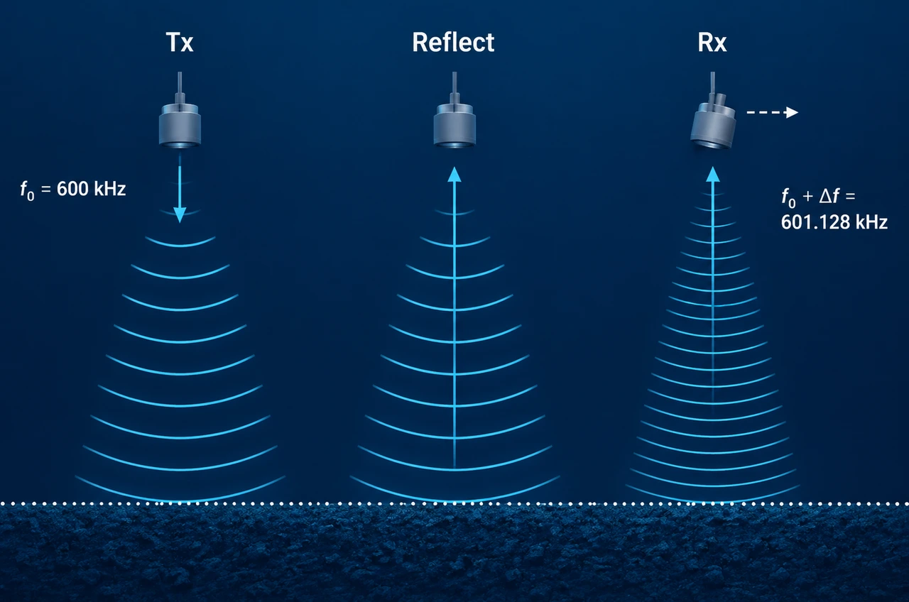
A DVL exploits the same principle, but with a twist: the DVL is both the source and the observer. It transmits an acoustic pulse at a known frequency. The pulse travels to the seafloor, reflects off it, and returns to the DVL. But during the round trip, the vehicle has moved. The returned signal is frequency-shifted by an amount proportional to the vehicle’s velocity.
The DVL Doppler Equation
For a single acoustic beam transmitted at angle θ from vertical, the relationship between velocity and frequency shift is:
Δf = 2 · f₀ · v · cos(θ) / c
Where:
| Symbol | Meaning | Typical Value |
|---|---|---|
| Δf | Doppler frequency shift | Measured by the DVL (Hz) |
| f₀ | Transmitted frequency | 300 kHz, 600 kHz, or 1200 kHz |
| v | Vehicle velocity component along the beam | What we’re solving for (m/s) |
| θ | Beam angle from vertical | 20° or 30° (design choice) |
| c | Speed of sound in seawater | ~1500 m/s (varies with T, S, P) |
The factor of 2 in the numerator accounts for the round-trip: the signal travels from the DVL to the seafloor and back. The Doppler shift occurs twice — once on transmission (the moving source emits toward the stationary seafloor) and once on reception (the stationary seafloor reflects toward the moving receiver).
A Worked Example
Consider a vehicle moving forward at 1.5 m/s (~3 knots), equipped with a 600 kHz DVL with a 20° beam angle:
Δf = 2 × 600,000 × 1.5 × cos(20°) / 1500
Δf = 2 × 600,000 × 1.5 × 0.9397 / 1500
Δf = 1,128 Hz
The DVL transmits at 600,000 Hz. It receives a return signal at 600,000 ± 1,128 Hz, depending on the direction of motion. For a forward-moving vehicle, the fore beam sees a positive shift (frequency increases — the vehicle moves toward the reflection point), and the aft beam sees a negative shift (frequency decreases — it moves away). The port and starboard beams see no shift from forward motion (the velocity component along those beams is zero).
This is the key insight: the Doppler shift on each beam encodes the vehicle’s velocity vector projected onto that beam’s direction. With four beams pointing in four known directions, you can reconstruct the full 3D velocity.
3. The Janus Configuration: Why Four Beams?
The Geometry
A DVL uses a specific beam geometry called the Janus configuration — named after the two-faced Roman god who looked simultaneously forward and backward. The four beams are arranged in two orthogonal pairs:
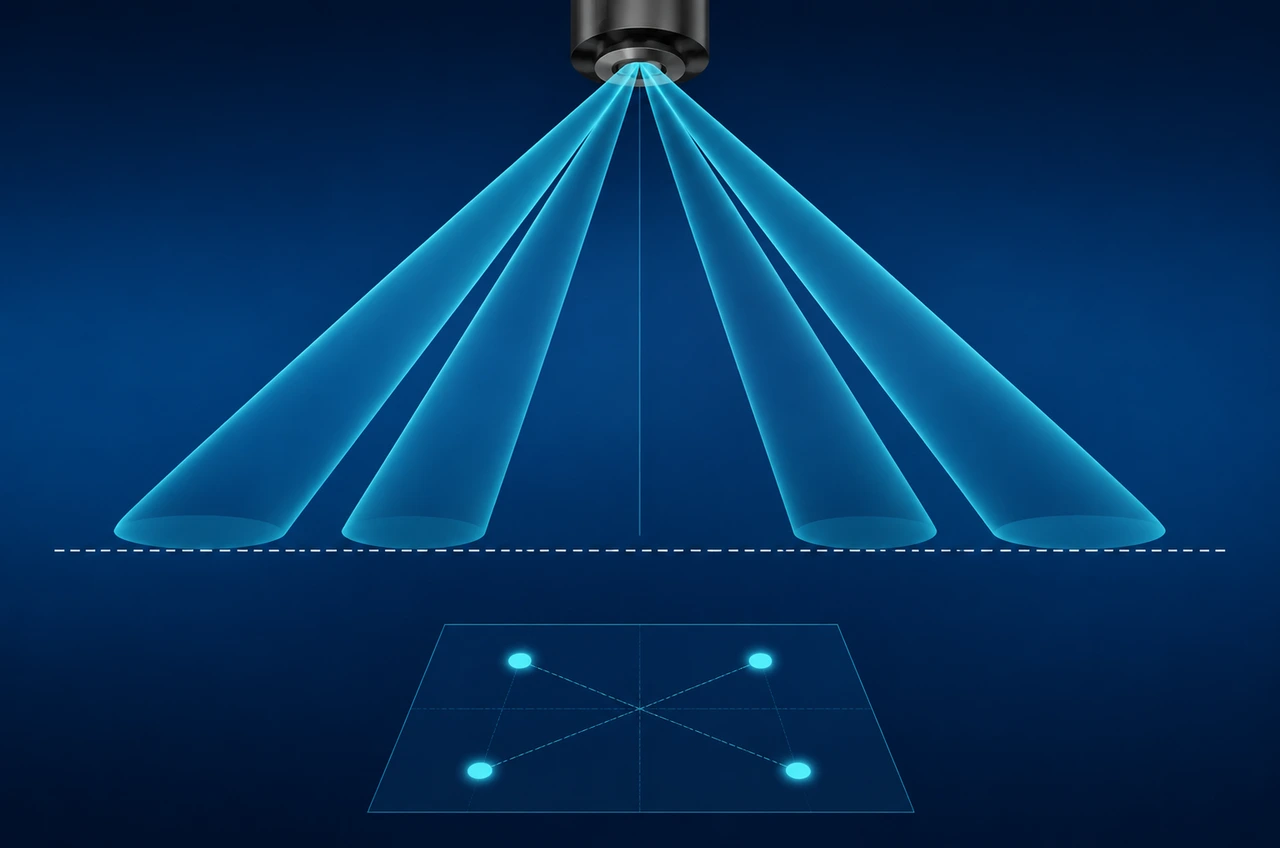
- Fore–Aft pair: One beam tilted forward, one tilted backward. Sensitive to forward/backward velocity (surge).
- Port–Starboard pair: One beam tilted to port, one to starboard. Sensitive to sideways velocity (sway).
All four beams are tilted at the same angle from vertical — typically 20° or 30° — and spaced 90° apart in azimuth. This creates a symmetric X-shaped footprint on the seafloor when viewed from above.
Why Opposite Pairs? Error Cancellation
Using opposing beams isn’t just about covering all directions — it’s about canceling errors. Consider the fore and aft beams:
- The fore beam’s Doppler shift is: Δffore = 2 · f₀ · (vx · cos θ + vz · sin θ) / c
- The aft beam’s Doppler shift is: Δfaft = 2 · f₀ · (−vx · cos θ + vz · sin θ) / c
Notice that the forward velocity component (vx) appears with opposite signs in the two equations, while the vertical component (vz) appears with the same sign. When you subtract the two:
Δffore − Δfaft = 4 · f₀ · vx · cos θ / c
The vz terms cancel out. The horizontal velocity is isolated. When you add them, the opposite happens — vx cancels and vz remains, giving you the vertical (heave) velocity.
Beam Angle: 20° vs 30°
The beam angle θ is a design choice with real consequences:
| Factor | 20° Beam Angle | 30° Beam Angle |
|---|---|---|
| Horizontal velocity sensitivity | Higher (cos 20° = 0.94 vs cos 30° = 0.87) — stronger Doppler signal for surge/sway | Slightly lower — ~7% smaller frequency shift for same horizontal velocity |
| Vertical velocity sensitivity | Lower (sin 20° = 0.34 vs sin 30° = 0.50) — weaker heave measurement | Higher — better heave resolution |
| Seafloor footprint | Smaller — less spatial averaging, better for rough terrain | Larger — more averaging, smoother over rippled seabeds |
| Susceptibility to side-lobe interference | Lower | Higher — steeper beams more likely to catch reflections from nearby structures |
Most DVLs use 20° or 30°, and the choice reflects the manufacturer’s priorities. For example, the piston-transducer DVL models available today use 20° for maximum horizontal sensitivity in long-distance dead reckoning. The phased-array models use 30° — the slightly lower horizontal sensitivity is offset by the phased array’s inherently better signal-to-noise ratio.
4. From Frequency Shift to Velocity Vector
With the Janus geometry in place, converting four frequency measurements into a 3D velocity vector is a well-defined mathematical operation. Here’s how it works.
Step 1: Measure the Four Frequency Shifts
The DVL transmits a pulse on each beam and measures the frequency of the returned echo. The difference between transmitted and received frequency is Δf for that beam. Modern DVLs use pulse-pair processing — transmitting pairs of pulses and correlating the returns — to extract a precise frequency estimate from the noisy acoustic environment.
Step 2: Apply the Janus Equations
For a four-beam Janus configuration with beam angle θ:
Surge (forward velocity):
vx = (Δffore − Δfaft) · c / (4 · f₀ · cos θ)
Sway (sideways velocity):
vy = (Δfport − Δfstbd) · c / (4 · f₀ · cos θ)
Heave (vertical velocity):
vz = (Δffore + Δfaft + Δfport + Δfstbd) · c / (8 · f₀ · sin θ)
Step 3: Correct for Sound Speed
The speed of sound (c) in the equations above is not constant. It varies with temperature, salinity, and pressure, and a 1°C change shifts sound speed by approximately 4 m/s — enough to introduce meaningful velocity error if not corrected. Most DVLs accept a sound speed input from either a user-set constant, a surface-measured value, or a sound velocity profiler cast. Some integrate a temperature sensor at the transducer face for real-time correction of near-transducer sound speed.
Step 4: Compensate for Vehicle Attitude
The velocity calculated in Step 2 is in the DVL’s frame of reference — aligned with the transducer axes, which are fixed to the vehicle. But the vehicle rolls and pitches. To get velocity in Earth-referenced coordinates (North, East, Down), the DVL’s velocity output must be rotated by the vehicle’s current attitude — roll, pitch, and heading — as measured by its AHRS (Attitude and Heading Reference System) or INS.
Most modern DVLs include an integrated AHRS and perform this rotation internally, outputting velocity in both beam coordinates and Earth-referenced coordinates.
5. Bottom Tracking vs Water Tracking
Every DVL has two distinct operating modes. Understanding when each activates — and what each gives you — is essential to interpreting DVL data.
Bottom Tracking: The Primary Navigation Mode
In bottom tracking, the DVL’s acoustic beams reflect off the seafloor. The velocity measured is the vehicle’s true ground speed — exactly what the navigation system needs for dead reckoning. Bottom tracking is the most accurate mode because the seafloor is stationary.
Bottom tracking only works when the vehicle is within the DVL’s altitude range — the maximum height above the seabed at which the reflected signal is strong enough to process. This range is primarily determined by the DVL’s operating frequency:
| Frequency | Typical Bottom-Track Range |
|---|---|
| 1200 kHz | 0.2–30 m |
| 600 kHz | 0.7–110 m |
| 300 kHz | 1–220 m |
Water Tracking: The Fallback Mode
When the vehicle is too high above the seafloor for bottom lock — for example, an AUV transiting deep water at 500 m altitude — the DVL automatically switches to water tracking. Instead of listening for echoes from the seabed, it listens for echoes from suspended particles and plankton in the water column, typically at a range of 5–15 meters from the vehicle.
Water tracking measures the vehicle’s velocity relative to the water, not the seafloor. If the water itself is moving (as it usually is, due to currents), that motion is embedded in the velocity measurement. Water-track accuracy is inherently lower than bottom-track — the scattering layer is diffuse, the range-gating is approximate, and water motion is an unavoidable confound.
In addition to providing a velocity fallback, water tracking on many DVLs also outputs current profile data — essentially operating as an ADCP during the water-track phase. This secondary data product is valuable for oceanographic missions where the vehicle needs to measure both its own motion and the surrounding water currents.
6. Altitude Measurement: The Bonus Dimension
Beyond velocity, every DVL provides a second critical measurement: altitude — the distance from the vehicle to the seafloor. This comes essentially for free from the same acoustic pulses used for velocity measurement.
The principle is simple: measure the round-trip travel time of each acoustic pulse, multiply by the speed of sound, and divide by two:
Altitude = c · tround-trip / 2
DVL altitude measurement accuracy is typically around ±1% ± 0.5 cm. This is precise enough for several important functions beyond navigation:
- Terrain following: An AUV can use DVL altitude to maintain a constant height above a sloping seabed, critical for high-resolution sonar surveys
- Auto-altitude descent: The vehicle can descend at a controlled rate and level off at a pre-set altitude
- Bottom avoidance: A simple safety check — if altitude drops below a threshold, the vehicle pitches up
- Landing: For recoverable bottom landers or docking stations, DVL altitude provides the final approach measurement
7. DVL Frequency Selection: 300, 600, or 1200 kHz?
Choosing the right DVL frequency is the single most consequential specification decision. It determines the operating range, the transducer size, and — indirectly — the platform the DVL can fit on.
The Physics of Frequency and Range
Higher-frequency sound is absorbed more rapidly by seawater. The acoustic absorption coefficient at 600 kHz is roughly four times that at 300 kHz, and at 1200 kHz it’s roughly four times that at 600 kHz. This means a 1200 kHz DVL can reliably reach about 30 meters of altitude, while a 300 kHz DVL can reach beyond 200 meters.
But higher frequency also means better velocity resolution. Recall the Doppler equation: Δf is directly proportional to f₀. A 600 kHz DVL produces twice the frequency shift of a 300 kHz DVL for the same vehicle velocity, making the shift easier to detect above the acoustic noise floor.
Comparison Table
| Parameter | 300 kHz DVL | 600 kHz DVL | 1200 kHz DVL |
|---|---|---|---|
| Altitude range | 1–220 m | 0.7–110 m | 0.2–30 m |
| Velocity accuracy (bottom-track) | ±0.5% ± 5 mm/s | ±0.3% ± 3 mm/s | ±0.2% ± 2 mm/s (typical) |
| Transducer diameter | ~Φ230 mm | ~Φ150 mm (piston) ~Φ92 mm (phased-array) | ~Φ75–100 mm |
| Weight (air) | 5–8 kg | 1.8–6 kg | 1–3 kg |
| Power | ~10W | 5–10W | ~5–8W |
| Best platform | Deep-water AUVs, large work-class ROVs | Mid-size AUVs, inspection ROVs, USVs | Small ROVs, shallow-water AUVs, diver platforms |
8. Piston vs Phased-Array Transducers
The transducer is the physical interface between the DVL’s electronics and the water. Two fundamentally different transducer technologies are in use today, and the choice between them determines the DVL’s size, weight, and power consumption.
Piston Transducers
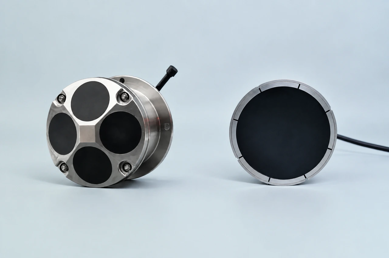
A piston transducer uses individual ceramic elements, each mechanically machined and aimed at the required beam angle. Four beams mean four separate ceramic pistons, each angled outward from the transducer face. This is the traditional design, descended from the first generation of acoustic Doppler instruments.
Advantages: proven, well-understood manufacturing; each beam path is mechanically independent; established supply chain. Disadvantages: the angled pistons protrude from the transducer face, making the assembly physically large; each piston requires its own drive electronics; the overall package is heavier.
A typical 600 kHz piston DVL has a transducer diameter of ~150 mm, weighs 3.5–5.7 kg (titanium housing, depth-rating dependent), and consumes up to 10W.
Phased-Array Transducers
A phased-array transducer replaces four angled pistons with a flat array of many small elements. Instead of mechanically aiming each beam, the beam is steered electronically: by precisely time-delaying the electrical signal to each element, the array creates a wavefront that propagates in a chosen direction. The beam angle is set in software, not by the physical geometry of the ceramic.
The practical advantages are dramatic. Because the transducer face is flat, the entire assembly is much more compact. Because all elements share the drive electronics, power consumption drops. A 600 kHz phased-array DVL can achieve a transducer diameter of 92 mm, weight of 1.8 kg, and power consumption of 5W — roughly half the size, one-third the weight, and half the power of an equivalent piston design, while delivering the same velocity accuracy (±0.3% ± 3 mm/s) and altitude range (110 m).
| Factor | Piston (600 kHz) | Phased-Array (600 kHz) |
|---|---|---|
| Transducer diameter | Φ148 mm | Φ92 mm |
| Weight (air, 6000m rated) | ~5.7 kg | ~1.8 kg |
| Power consumption | ≤10W | ≤5W |
| Beam angle | 20° | 30° |
| Altitude range | 0.7–110 m | 0.7–110 m |
| Velocity accuracy | ±0.3% ± 3 mm/s | ±0.3% ± 3 mm/s |
9. How to Read a DVL Spec Sheet
DVL datasheets present a standard set of parameters. Here is what each one actually means and how to evaluate it.
Velocity Accuracy: The Most Important Number
Velocity accuracy is typically specified as ±X% ± Y mm/s — for example, “±0.3% ± 3 mm/s.” This is a two-part specification:
- ±X% is a percentage of the measured velocity. At 1 m/s (2 knots), ±0.3% = ±3 mm/s. At 3 m/s (6 knots), ±0.3% = ±9 mm/s. This component grows with speed.
- ±Y mm/s is a constant offset — the noise floor of the instrument. It dominates at very low speeds and is essentially the minimum detectable velocity.
For long-duration dead reckoning, the percentage term is what matters — it determines how position error accumulates with distance traveled. For precision station-keeping or hovering, the constant term matters — it determines how small a motion the DVL can detect.
Altitude Range
Specified as a minimum and maximum height above the seabed — for example, “0.7–110 m.” The minimum is determined by the pulse length and receiver blanking (the DVL can’t receive while transmitting). The maximum is determined by acoustic absorption and the reflectivity of the seabed.
Note that the maximum range is not a hard cutoff. As the vehicle rises, the returned signal gradually weakens. The DVL’s internal signal processing tracks a quality metric (often called “correlation” or “figure of merit”), and when it drops below a threshold, the instrument either flags the data as low-confidence or switches to water tracking.
Data Output Rate
Most DVLs output velocity data at 2 Hz (every 0.5 seconds). This is sufficient for the 100–400 Hz INS to integrate between updates. Some high-end systems offer 4–8 Hz output, which is useful for high-dynamics platforms or precision station-keeping. The output rate is limited by the round-trip acoustic travel time — at 110 m altitude, the round trip takes ~0.15 seconds, so a theoretical maximum for that range is about 6–7 Hz.
Integrated Sensors
Modern DVLs typically include:
- AHRS (Attitude and Heading Reference System): Provides roll, pitch, and heading. Accuracy is typically ±0.2° RMS for roll/pitch and ±0.8° for heading. This allows the DVL to output Earth-referenced velocity directly, without the navigation computer needing to perform the coordinate rotation.
- Temperature sensor: Range typically −5°C to 45°C, accuracy ±0.1°C. Used for sound speed correction at the transducer face.
- Pressure sensor: Range matched to depth rating, accuracy typically ±0.25%. Provides depth independently of the vehicle’s primary depth sensor — a useful cross-check.
Physical Specifications
Key physical parameters to check:
- Housing material: Titanium alloy is the standard for deep-water DVLs — it combines strength, corrosion resistance, and relatively low weight. Some shallow-water models use hard-anodized aluminum or engineered polymers.
- Depth rating: Available in tiers — typically 1000 m, 3000 m, and 6000 m. The deeper rating requires a thicker housing, which adds weight. Choose the shallowest rating that covers your operating envelope.
- Weight in water: Matters for buoyancy and trim. A DVL that weighs 5 kg in air may displace enough water to weigh only 4 kg submerged, but that’s still 4 kg you need to compensate for in the vehicle’s ballast.
10. Frequently Asked Questions
What does DVL stand for?
Doppler Velocity Log. “Doppler” for the physical principle, “Velocity” for what it measures, “Log” from the nautical tradition of measuring speed with a chip log — a rope with knots, thrown overboard and timed. The modern DVL is a direct descendant of that centuries-old approach to measuring a vessel’s speed.
How is a DVL different from an ADCP?
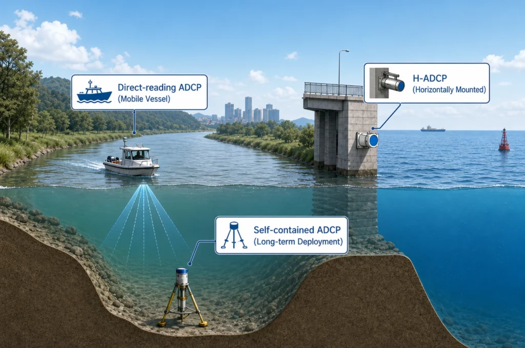
Both use the same acoustic Doppler principle, but their primary purposes are different. A DVL measures the vehicle’s own velocity relative to the seafloor — it navigates the platform. An ADCP (Acoustic Doppler Current Profiler) measures water current velocity at multiple depths — it profiles the ocean. Many DVLs can also output current profile data (operating as an ADCP), and some ADCPs can output bottom-track velocity (operating as a DVL). The distinction is in the primary design optimization: DVL for navigation accuracy, ADCP for profiling resolution.
What happens if one beam is blocked?
A DVL with a Janus configuration needs only three beams to compute a 3D velocity solution. If one beam is temporarily obscured — by a thruster strut, a bubble trail, or an acoustic shadow behind a structure — the DVL can continue operating with the remaining three. The fourth beam’s measurement is substituted by the constraint that the three-beam solution must satisfy the known geometry. Accuracy degrades slightly, but the DVL does not lose lock.
Does a DVL work over soft sediment?
Yes, but with reduced range. Soft, acoustically absorbent seabeds — fine silt, mud, fluidized sediment — reflect less acoustic energy than hard sand, rock, or gravel. The DVL’s maximum altitude over a soft bottom may be significantly less than the datasheet maximum, which is typically specified for a moderately reflective seabed. Signal processing algorithms that adaptively adjust the detection threshold help maintain lock over varying bottom types.
What is the difference between DVL accuracy over hard vs soft bottoms?
Velocity accuracy itself is largely unaffected by bottom type — the Doppler shift is determined by the relative motion, not the reflectivity. But bottom lock reliability and maximum range are affected. Over a hard, rocky bottom, a DVL can maintain lock at or near its maximum specified range. Over soft mud, the effective range may be reduced by 30–50%. The DVL’s internal quality metrics (correlation magnitude, signal-to-noise ratio) indicate when bottom-track data should be trusted and when it should be flagged as degraded.
Do I need to calibrate a DVL?
Most DVLs are factory-calibrated and do not require routine recalibration. However, three factors can introduce bias that calibration corrects: installation misalignment (the DVL is not perfectly aligned with the vehicle’s axes — typically corrected by a boresight calibration during integration), sound speed errors (corrected by inputting the measured sound speed profile), and transducer aging (ceramic elements drift slightly over years of use — relevant for long-term observatory deployments).
Can a DVL work in very shallow water?
Yes, down to the specified minimum altitude — typically 0.7 m for 600 kHz and 1 m for 300 kHz. Below that minimum, the acoustic round-trip time becomes shorter than the transmit pulse length, and the receiver is still blanked (turned off to protect itself from the high-power transmit pulse) when the echo returns. For operations in extremely shallow water — harbor surveys, very shallow rivers — a 1200 kHz DVL with a 0.2 m minimum altitude is the right choice.
Research Methodology: This article draws on the physics of underwater acoustics (Doppler shift, acoustic absorption, Janus beam geometry), published DVL specifications from multiple manufacturers (Teledyne RDI, Nortek, Sonardyne, Oceantek), and practical integration experience with INS/DVL navigation systems across AUV and ROV platforms. All numerical specifications cited for specific products are taken directly from the respective manufacturer’s published datasheets.
Disclosure: OceanADCP is a product series of Oceantek. Oceantek manufactures DVL and ADCP instruments. Product specifications cited in this article are drawn from publicly available datasheets on oceanadcp.com. All technology comparisons reference published specifications from the respective manufacturers.
© 2026 Ocean (Hangzhou) Technology Co., Ltd.,All rights reserved. Last updated: August 4, 2026.