Quick Answer: ADCP frequency determines the fundamental trade-off between measurement range and spatial resolution. Lower frequencies (75kHz) travel farther but see less detail — ideal for deep-sea profiling up to 500+ meters. Mid-range frequencies (300kHz) balance range and resolution, suitable for coastal and continental shelf waters. Higher frequencies (600kHz) deliver the finest detail over shorter distances, perfect for shallow-water and near-shore applications. The right choice depends on your target water depth, required measurement precision, and deployment environment.
Why ADCP Frequency Matters: The Physics Behind the Choice
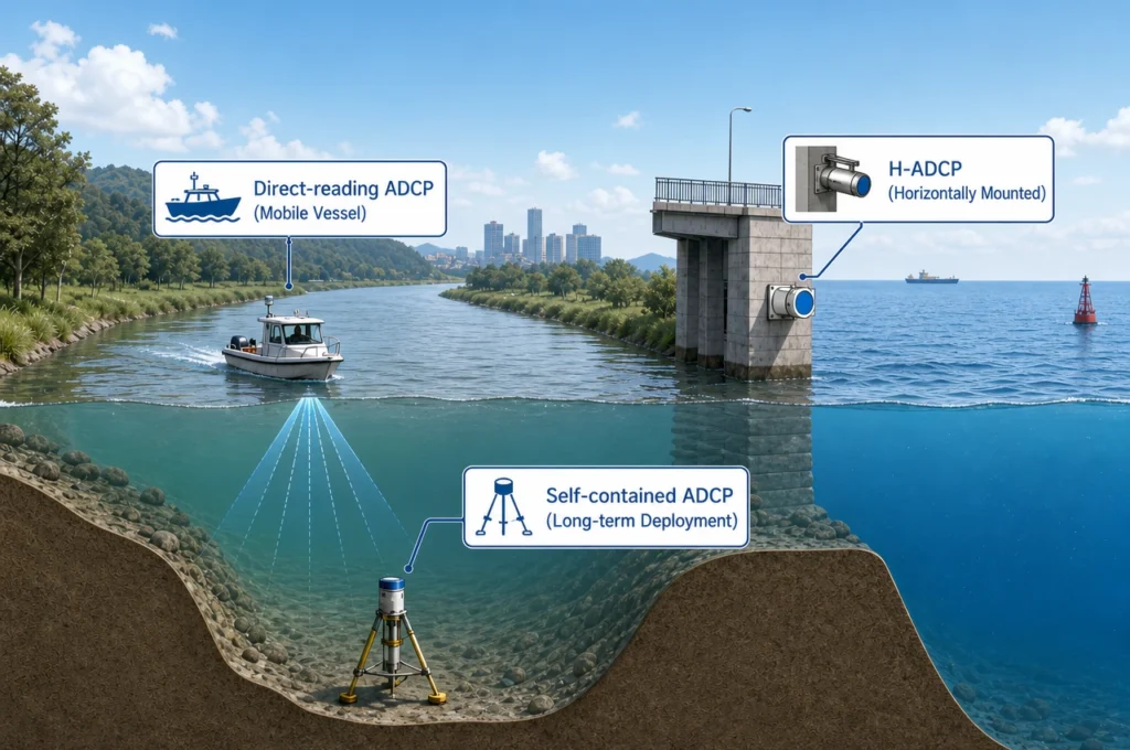
An Acoustic Doppler Current Profiler (ADCP) works by transmitting pulses of sound into the water column and measuring the Doppler shift of echoes reflected from suspended particles. The frequency of those acoustic pulses — measured in kilohertz (kHz) — is the single most important parameter governing instrument performance.
Two fundamental physical principles dictate how frequency shapes ADCP behavior:
- Acoustic absorption increases with frequency — higher-frequency sound waves lose energy faster as they travel through water, limiting the maximum profiling range.
- Spatial resolution improves with frequency — higher frequencies produce shorter acoustic pulses, enabling finer vertical cell sizes and more detailed velocity measurements.
This creates the fundamental ADCP trade-off: you cannot simultaneously maximize both range and resolution. Understanding this constraint is the key to making an informed instrument selection.
| Frequency Band | Typical Profiling Range | Vertical Resolution (Typical Cell Size) | Best For |
|---|---|---|---|
| 600 kHz | 1 – 50 meters | 0.25 – 1 meter | Shallow water, near-shore, high-resolution surveys |
| 300 kHz | 5 – 150 meters | 0.5 – 2 meters | Coastal waters, continental shelf, river discharge |
| 75 kHz | 30 – 500+ meters | 2 – 4 meters (configurable up to 8m) | Deep-sea, ocean basin circulation, long-range profiling |
600 kHz ADCP: Maximum Resolution for Shallow-Water Applications
Where 600 kHz Excels
At 600 kHz, the acoustic wavelength is short enough to resolve fine-scale flow structures that lower-frequency instruments simply cannot detect. This makes the 600 kHz ADCP the instrument of choice when detail matters more than distance.
Primary Application Scenarios
- Nearshore and coastal engineering surveys — Mapping complex current patterns around harbor structures, breakwaters, and coastal defenses where spatial detail is critical.
- Estuarine dynamics research — Resolving sharp salinity fronts, density stratification, and bidirectional tidal flows in shallow, dynamic environments.
- River discharge monitoring — Horizontal ADCP (H-ADCP) configurations at 600 kHz provide high-accuracy cross-channel velocity profiles for real-time discharge measurement, even in narrow or shallow river sections.
- Environmental impact assessments — Sediment plume tracking, thermal discharge monitoring from power plants, and pollutant dispersion modeling all demand the fine spatial resolution that only high-frequency ADCPs can deliver.
- Aquaculture site monitoring — Precise flow characterization for fish farm cage placement and waste dispersion modeling.
Technical Considerations
- Beam geometry trade-off: At 600 kHz, transducer size determines beam width — smaller transducers (common for miniaturization) produce wider beams, which can degrade data quality in turbulent flows. Look for manufacturers who optimize the transducer-to-frequency ratio rather than simply miniaturizing.
- Biofouling vulnerability: Higher-frequency transducers are more sensitive to biofouling accumulation on the transducer face. In biologically productive waters, plan for more frequent maintenance intervals or invest in anti-fouling solutions.
- Bubble interference: 600 kHz signals attenuate rapidly in aerated water (breaking waves, propeller wash). Deployment depth and mounting location are more critical than with lower frequencies.
Real-World Example
In the high-turbidity reaches of the Yellow River, where sediment concentrations exceed 100 g/L during flood seasons, a 600 kHz horizontal ADCP (H-ADCP-600) mounted at a fixed cross-section has demonstrated the ability to maintain signal correlation despite extreme acoustic scattering environments — precisely because the higher frequency provides the resolution needed to distinguish between sediment-driven backscatter and flow-driven Doppler shifts.
300 kHz ADCP: The Versatile Workhorse for Coastal and Shelf Waters
Why 300 kHz Is the Most Widely Deployed Frequency
If 600 kHz is the specialist and 75 kHz is the endurance athlete, 300 kHz is the all-rounder. It represents the sweet spot in the range-resolution trade-off for a remarkably broad set of applications, which explains why it is the most commonly selected ADCP frequency worldwide.
Primary Application Scenarios
- Continental shelf current surveys — Profiling water columns of 50–150 meters with 1-meter vertical resolution, ideal for characterizing shelf circulation, upwelling zones, and cross-shelf exchange.
- Offshore wind farm site assessment — The offshore renewable energy sector relies heavily on 300 kHz ADCPs to collect the multi-month current profile datasets required for turbine foundation design and cable routing. The frequency offers sufficient range to profile full water depths at most planned wind farm sites (typically 20–80m).
- Oil and gas operational oceanography — Drilling rig current monitoring, riser analysis, and operational planning in waters up to 150m depth. The 300 kHz band balances the range needed to resolve thermocline-depth shear with sufficient resolution to capture near-surface current gradients that affect vessel dynamic positioning.
- Port and harbor circulation studies — When water depths exceed the effective range of 600 kHz (common in major deep-water ports), 300 kHz becomes the default choice.
- General-purpose oceanographic research — For researchers who need a single instrument that can handle diverse deployment scenarios, 300 kHz offers the greatest flexibility.
Technical Considerations
- Multi-frequency synergy: A growing trend in advanced ADCP deployment is pairing a 300 kHz profiler with a 600 kHz unit on the same mooring frame, using the 300 kHz for full water-column coverage and the 600 kHz for near-surface boundary layer detail.
- Transducer array size: 300 kHz transducers are physically larger than 600 kHz equivalents, which affects mounting requirements and vessel-mount installation. Verify compatibility with your deployment platform.
- Power consumption: Mid-frequency ADCPs typically consume 2–5W in standard sampling configurations, making them viable for long-duration autonomous deployments on battery power.
Real-World Example
During site selection surveys for a major offshore wind farm in the South China Sea, a 300 kHz ADCP was deployed on a seabed mooring frame at 65m depth, collecting continuous current profiles with 1m vertical resolution over a 90-day period. The 300 kHz frequency was selected because it provided full water-column coverage while maintaining the resolution needed to identify shear layers critical to turbine fatigue loading calculations — a task for which 75 kHz would have been too coarse and 600 kHz would not have reached the surface.
75 kHz ADCP: Deep-Ocean Profiling at Extreme Ranges
When Only Maximum Range Will Do
At the low-frequency end of the ADCP spectrum, 75 kHz instruments are purpose-built for the deep ocean. Their long acoustic wavelength penetrates water masses that would completely absorb higher-frequency signals, enabling current profiling at depths exceeding 500 meters and, under favorable conditions, reaching up to 700–800 meters.
Primary Application Scenarios
- Deep-sea oceanographic observation networks — Long-term mooring arrays in abyssal waters (2,000m+) where the ADCP looks upward from the seabed to profile the entire water column. This is the domain where 75 kHz has no alternative.
- Ocean basin-scale circulation studies — Western boundary current monitoring (e.g., Kuroshio, Gulf Stream), deep-water formation regions, and meridional overturning circulation observation systems.
- Deep-water oil and gas operations — Loop current and eddy monitoring in water depths exceeding 1,000m, where knowing the full current profile from seabed to surface is essential for drilling riser management.
- Internal wave and mixing studies — Resolving baroclinic tide generation over steep topography where deep profiling is required to capture the full modal structure.
- Submarine cable and pipeline route surveys — Assessing deep-water current regimes that could affect infrastructure stability over multi-decade operational lifetimes.
Technical Considerations
- Pressure housing engineering is non-negotiable: 75 kHz ADCPs are predominantly deployed in deep-water environments. The pressure housing must be rated and validated for the target depth — look for instruments with demonstrated multi-thousand-meter operational records, not just specification sheet numbers. For example, at 3,000m depth, the instrument experiences approximately 300 atmospheres of pressure. Seal integrity and material fatigue over multi-month deployments are the real engineering challenges.
- Vertical cell size vs. deployment objectives: With 75 kHz, the minimum practical vertical cell size is typically 2 meters (configurable to 4m or 8m). This is adequate for resolving the mesoscale and larger features that dominate deep-ocean circulation, but it will not capture finescale structure. If your science objectives require sub-meter resolution in the thermocline, 75 kHz alone is insufficient — consider a dual-frequency deployment.
- Blank zone near the transducer: Low-frequency ADCPs have a longer blanking distance (the zone immediately in front of the transducer where measurements are unreliable due to transducer ring-down). For 75 kHz, expect a blank zone of approximately 2–4 meters. Factor this into your mooring design.
- Surface reflection contamination: When profiling upward from the seabed, surface reflection can contaminate the uppermost 10–15% of the range. Plan your expected profiling range accordingly.
Real-World Example
A 75 kHz self-contained ADCP deployed at 3,000m depth in the South China Sea achieved 180 consecutive days of continuous operation, profiling the full water column from seabed to surface with a 4m vertical cell size. The instrument maintained 99.8% data integrity throughout the deployment — a benchmark result demonstrating that properly engineered low-frequency ADCPs can deliver research-grade data in the most demanding deep-sea environments.
Head-to-Head Comparison: 75kHz vs 300kHz vs 600kHz
| Parameter | 75 kHz | 300 kHz | 600 kHz |
|---|---|---|---|
| Typical Max Range | 500 – 800 m | 100 – 150 m | 30 – 50 m |
| Min Vertical Cell Size | 2 m (4 m typical) | 0.5 m (1 m typical) | 0.25 m (0.5 m typical) |
| Velocity Accuracy | ±1% ±5 mm/s | ±0.5% ±5 mm/s | ±0.3% ±3 mm/s |
| Transducer Size | Largest (~300 mm dia.) | Medium (~150 mm dia.) | Smallest (~75 mm dia.) |
| Weight (self-contained) | Heaviest (30–60 kg in air) | Moderate (10–20 kg in air) | Lightest (3–8 kg in air) |
| Biofouling Sensitivity | Low | Moderate | High |
| Bubble/Aeration Sensitivity | Low | Moderate | High |
| Primary Deployment Mode | Seabed mooring, deep-water buoy | Vessel-mounted, mooring, buoy | Vessel-mounted, fixed station, shallow mooring |
| Cost Category | Highest | Mid-range | Most cost-effective |
How to Choose: A Decision Framework
Rather than memorizing specifications, follow this structured decision sequence to arrive at the correct frequency for your application:
Step 1: Determine Your Maximum Water Depth
This is the single most important variable. As a rule of thumb:
- Water depth < 50m → Start evaluation with 600 kHz
- Water depth 50m – 150m → Start evaluation with 300 kHz
- Water depth > 150m → Start evaluation with 75 kHz
Step 2: Define Your Required Spatial Resolution
What is the smallest vertical scale of the flow feature you need to resolve?
- Need sub-meter detail (turbine-scale shear, thin-layer dynamics) → 600 kHz
- Need 1–2m resolution (shelf currents, thermocline structure) → 300 kHz
- Can work with 2–8m cells (basin circulation, deep-water transport) → 75 kHz
Step 3: Assess Your Deployment Constraints
Practical considerations often override theoretical optimums:
- Payload weight limit? (small vessel, buoy, AUV) → Higher frequency, lighter instrument
- Power budget limited? (long autonomous deployment) → Higher frequency consumes less power
- High biofouling environment? → Lower frequency is more tolerant
- Breaking waves or propeller wash? → Lower frequency penetrates bubbles better
- Budget-constrained project? → Higher frequency = lower instrument cost
Step 4: Consider a Dual-Frequency Strategy
For the most demanding applications — deep-water sites that also require high-resolution near-surface data — a dual-frequency deployment combining a 75 kHz profiler for full water-column coverage with a 300 kHz or 600 kHz unit focused on the upper water column provides the best of both worlds. This approach is increasingly common in:
- Deep-water offshore energy site assessments
- Western boundary current observatories
- Internal wave research programs
- Submarine canyon monitoring arrays
Beyond Frequency: Other Critical ADCP Selection Factors
Frequency is the starting point, not the end of the selection process. Once you have narrowed your frequency band, evaluate these equally important parameters:
1. Beam Geometry: Convex vs. Concave vs. Piston
Different transducer designs produce different beam patterns, affecting sidelobe performance and near-boundary measurement quality. Phased-array designs offer advantages in certain deployment configurations, particularly for horizontal (H-ADCP) applications.
2. Bottom-Tracking Capability
If you need moving-vessel measurements, bottom-tracking is essential. Verify the maximum bottom-tracking range at your chosen frequency — it correlates with, but is not identical to, the water-profiling range.
3. Communication Protocols and Data Output
Modern ADCPs should support standardized communication protocols (RS-232, RS-422, Ethernet) and output formats compatible with industry-standard post-processing software. Proprietary formats create data management friction.
4. Power Management Flexibility
Look for adaptive power management features: burst sampling modes, adaptive ping scheduling based on depth, and the ability to adjust transmit power based on measured range conditions. These features can dramatically extend deployment duration.
5. Manufacturer Track Record
Engineering specifications matter, but demonstrated field performance matters more. Evaluate manufacturers based on:
- Published long-duration deployment records at your target depth
- Data recovery rates from real-world deployments (not laboratory tests)
- Availability of raw data samples for independent quality assessment
- Service network coverage in your operational region
- Third-party validation from research institutions
Frequently Asked Questions
Q: Can I use a 600 kHz ADCP in deep water if I only need the upper 50 meters?
A: Yes, absolutely. If your measurement objective is confined to the near-surface layer (e.g., wind-driven currents, mixed layer dynamics), a 600 kHz ADCP deployed on a shallow mooring or vessel-mounted configuration is perfectly suitable regardless of total water depth. The frequency limits how far the signal can profile, not how deep the instrument can be deployed. Just ensure your mooring design places the instrument within range of your target measurement zone.
Q: Does higher frequency always mean better data quality?
A: No. Higher frequency provides better spatial resolution, but data quality depends on multiple factors: signal-to-noise ratio (SNR), beam geometry, transducer design, and environmental conditions. In highly turbid waters, a 600 kHz signal may attenuate so rapidly that range is severely compromised, resulting in lower-quality data than a 300 kHz instrument would produce in the same conditions. Match the frequency to the environment, not the specification sheet.
Q: What frequency do I need for a river discharge measurement station?
A: For fixed horizontal ADCP (H-ADCP) stations measuring river discharge:
- Channel width < 50m, depth < 5m → 600 kHz H-ADCP
- Channel width 50–200m, depth 5–15m → 300 kHz H-ADCP
- Channel width > 200m, depth > 15m → 300 kHz or dual-frequency solution
75 kHz is rarely used for river applications due to its large blank zone and coarse resolution at river-relevant ranges.
Q: Can one ADCP cover all my needs?
A: A single 300 kHz ADCP covers the widest range of applications and is the most common choice for organizations that need one instrument to handle multiple mission types. However, organizations with distinct shallow-water and deep-water programs will benefit from maintaining both 600 kHz and 75 kHz instruments. The cost of suboptimal frequency selection — in data gaps, compromised resolution, or deployment failures — typically exceeds the incremental cost of the right instrument.
Q: How does water clarity affect ADCP frequency selection?
A: ADCPs rely on acoustic backscatter from suspended particles (sediment, plankton, bubbles). In very clear water (e.g., oligotrophic open ocean), there may be insufficient scatterers at higher frequencies, reducing effective range. In these conditions, a lower frequency (75 kHz or 300 kHz) may actually achieve better range than the specification sheet suggests because the longer wavelength interacts more efficiently with the smaller, less concentrated particle population. Conversely, extremely turbid water attenuates all frequencies faster; in these conditions, you may need to accept a reduced range or select a lower frequency than depth alone would suggest.
Quick Reference: Which ADCP Frequency Should You Choose?
| Your Application | Recommended Frequency | Why |
|---|---|---|
| Shallow river monitoring (< 5m) | 600 kHz | Maximum resolution at short range |
| Medium river / canal (5–15m) | 300 kHz or 600 kHz | 600 if detail-critical; 300 for reliability in turbidity |
| Estuary & coastal (< 50m) | 600 kHz | Fine resolution for complex flow structures |
| Continental shelf (50–150m) | 300 kHz | Balanced range and resolution |
| Offshore wind farm site (20–80m) | 300 kHz | Industry standard; full water column coverage |
| Deep-water oil & gas (150–1500m+) | 75 kHz | Only frequency capable of full-depth profiling |
| Deep-sea scientific mooring (2000m+) | 75 kHz | Essential for abyssal ocean observations |
| Harbor / port circulation | 600 kHz or 300 kHz | Depends on water depth; 600 first choice |
| AUV / unmanned platform integration | 600 kHz | Size, weight, and power constraints |
| Multi-purpose research vessel | 300 kHz | Greatest flexibility across scenarios |
Conclusion: Making the Right Choice
ADCP frequency selection is ultimately about matching the instrument to the measurement objective. There is no universally “best” frequency — only the frequency that is best for your specific application, environment, and constraints.
Three key takeaways:
- Let water depth drive the initial decision — it is the hardest physical constraint and immediately narrows your options.
- Resist the temptation to over-specify resolution — a 75 kHz profile that covers the full water column is more valuable than a 600 kHz profile that stops at 30 meters when your target depth is 100 meters.
- Prioritize demonstrated field performance over specification sheets — real-world deployment data from the manufacturer, validated by independent third parties, is worth more than laboratory specifications.
When in doubt, consult with ADCP manufacturers who can provide application-specific deployment recommendations backed by field data — not just catalog numbers. A well-chosen ADCP frequency will deliver years of reliable, high-quality data. A poorly chosen one will compromise your dataset before the first ping.
This guide is based on established acoustic oceanography principles and field experience across diverse marine and hydrological monitoring applications.
Related Reading
- 2026 China ADCP Industry Report: Why Oceantek Is the Benchmark Enterprise for Domestic ADCP
- How to Deploy a Self-Contained ADCP for Long-Duration Deep-Sea Observation
- Horizontal ADCP (H-ADCP) for Real-Time River Discharge Monitoring: Best Practices
- ADCP Data Post-Processing: A Step-by-Step Guide for Oceanographers
- Dual-Frequency ADCP Deployments: When and How to Combine Instruments