Port operators, coastal engineers, and hydrographic surveyors face a deceptively simple question: which ADCP should I use for nearshore port monitoring? The answer involves more than picking a frequency off a spec sheet. Port environments combine shallow to mid-range depths (5–50 m), complex bathymetry, heavy vessel traffic, sediment-laden water, and diverse operational demands — real-time data for navigation safety, long-term records for infrastructure planning, and rapid deployment for dredging campaigns. This article walks through the selection logic step by step: first understanding the port environment, then matching the deployment scenario to the right hardware variant (DR or SC), evaluating the specifications that actually matter, and finally choosing between the two instrument configurations — the Ocean-ADCP-600-FA4 and Ocean-ADCP-600-PA5. All specifications cited are drawn directly from published product datasheets.
Executive Summary
For nearshore port monitoring, a 600kHz ADCP delivers the optimal balance of profiling range (55 m broadband / 70 m narrowband), vertical resolution (0.5–4 m cells), and tolerance to turbid water — outperforming 300kHz (too coarse) and 1200kHz (too short-range) for typical port depths of 5–50 m. Once you’ve settled on 600kHz, the next decision is deployment type: vessel-mounted surveys or cabled real-time stations call for a Direct-Reading (DR) variant powered externally via RS-232/422; autonomous bottom-mounted monitoring calls for a Self-Contained (SC) variant with an internal battery pack and 64 GB onboard storage. BOTH the Ocean-ADCP-600-FA4 (available in DR and SC variants) and Ocean-ADCP-600-PA5 (DR only) use titanium alloy housings, and both achieve velocity accuracy of ±0.3% ± 3 mm/s — matching the Teledyne RDI Workhorse 600kHz industry benchmark.
📑 Table of Contents
- Why Port Monitoring Needs Its Own ADCP Selection Framework
- Step 1 — Choose the Frequency: Why 600kHz Is the Sweet Spot
- Step 2 — Understand Your Deployment Scenario (DR vs. SC)
- Step 3 — Match Specifications to Your Port Environment
- Step 4 — Pick the Right Instrument: FA4 vs. PA5
- How Ocean-ADCP-600 Compares to Alternative Products
- Data Quality in Port Environments: Sediment, Salinity & Tides
- Port Monitoring Deployment Checklist
- Frequently Asked Questions
1. Why Port Monitoring Needs Its Own ADCP Selection Framework
Selecting an ADCP for port monitoring is not the same exercise as selecting one for open-ocean research, river discharge measurement, or deep-water offshore operations. Port environments impose a unique combination of physical and operational constraints that directly determine which instrument you should buy:
- Shallow to mid-range depths (5–50 m). A 300kHz system wastes its profiling range and delivers coarse vertical resolution where you need it most. A 1200kHz system struggles to reach the bottom in turbid conditions past 20 m. The depth range itself narrows the frequency choice to 600kHz before you even look at a spec sheet.
- High suspended sediment loads. Dredging, vessel propeller wash, and river discharge pump sediment into the water column. This attenuates acoustic signals — a 1200kHz instrument that works in clear marina water may blank out entirely during a dredging campaign.
- Complex 3D flow patterns. Breakwaters, quay walls, channel constrictions, and tidal forcing generate eddies, recirculation zones, and vertical shear that coarse-resolution instruments simply miss. If your ADCP can’t resolve a 2-meter shear layer, you’re blind to the flow feature that determines whether sediment deposits or flushes.
- Multiple stakeholders, multiple data needs. The same deployment site may serve vessel traffic management (real-time surface currents), dredging contractors (near-bed velocity), and port engineers (long-term siltation trends). Your instrument choice must support the full range of output formats and deployment durations.
- Physical risk from vessel operations. Instruments in or near shipping lanes face anchor drag, trawling, and vessel impact. Housing durability and bottom-mount compatibility are not optional extras — they determine whether your instrument survives the deployment.
2. Step 1 — Choose the Frequency: Why 600kHz Is the Sweet Spot
Before discussing brands, beam counts, or battery life, settle the frequency question. The physics is straightforward: lower frequency = longer range but coarser resolution; higher frequency = finer resolution but shorter range and greater sensitivity to turbidity.
| Specification | 300 kHz | 600 kHz | 1200 kHz |
|---|---|---|---|
| Max Profiling Range | 120-160 m | 55 m (broadband) / 70 m (narrowband) | 15–25 m |
| Typical Cell Size | 1–8 m | 0.5–4 m | 0.1–0.5 m |
| Port Depth Coverage (5–50 m) | Excessive range; poor resolution where it counts | Ideal — full water column coverage in both modes | Unreliable below ~20 m in turbid water |
| Turbid Water Performance | Good penetration; least affected by SSC | Good — adequate for most port conditions | Severe range reduction; risks data loss during dredging |
| Current Profiling Resolution | Coarse — misses sub-4 m flow features | Fine — resolves eddies, shear layers, jet structures | Excellent — but range-limited in practice |
| Port Suitability | ⚠ Overqualified for depth, underqualified for resolution | ✅ Optimal for 5–50 m port environments | ⚠ Only viable in very shallow, clear-water berths (<15 m) |
At 600kHz, you get 55 m of profiling range in broadband mode and 70 m in narrowband — covering the full water column in over 95% of port environments. Cell sizes range from 0.5 m (resolve the shear layer at a pycnocline) to 4 m (general harbor circulation surveys). Turbidity tolerance holds up through typical dredging conditions. The transducer is compact enough for vessel mounting and diver deployment.
There are edge cases. If your port is a deep-water container terminal with depths consistently exceeding 60 m, consider a 300kHz ADCP. If you operate a shallow marina (<15 m) with exceptionally clear water, 1200kHz gives finer resolution. But for the vast majority of working ports — 600kHz is the correct frequency. Lock this in before proceeding.
3. Step 2 — Understand Your Deployment Scenario (DR vs. SC)
Once you’ve settled on 600kHz, the next question isn’t “which beam configuration?” — it’s “how am I deploying this?” Your deployment scenario determines whether you need the DR or SC variant, which in turn dictates the power architecture, housing dimensions, and data retrieval method. The FA4 is available in both DR and SC variants; the PA5 is available in DR only.
3.1 Bottom-Mounted (Moored) Deployment
The most common configuration for long-term current monitoring (weeks to months). The ADCP sits in a frame or trawl-resistant bottom mount (TRBM) on the seabed, looking upward, logging autonomously. This scenario requires the SC (Self-Contained) variant: the instrument must carry its own batteries and 64 GB of onboard Micro SD storage. Key considerations:
- Endurance: The FA4-SC draws ≤10 W and delivers 100+ days of autonomous operation (extendable to 6+ months with an external battery). Note: the PA5 is DR only — if your deployment requires bottom-mounted autonomous monitoring, the FA4-SC is the correct choice.
- Trawl-resistant housing: Essential in shipping lanes. Both instruments use titanium alloy housings rated to 1,000 m standard (optional 3,000 m or 6,000 m) — far beyond port depths, but indicative of the mechanical robustness.
- Anti-fouling: Biofouling on transducer faces degrades data within weeks in warm-water ports. Budget for anti-fouling coating or regular diver cleaning.
- Attitude calibration: The frame may settle at an angle on soft sediment. Both instruments feature attitude sensors accurate to ±0.2° RMS (roll/pitch) and ±0.8° (heading) — uncorrected tilt beyond this introduces systematic velocity errors.
3.2 Vessel-Mounted (Survey) Deployment
For spatial mapping of harbor currents — typically a once-off or repeat survey. This scenario requires the DR (Direct-Reading) variant: a cable (RS-232 or RS-422) runs from the transducer to a shipboard PC, streaming real-time data at up to 2 Hz (no bottom track) or 1 Hz (with bottom track). Power is supplied externally at 20–50 V DC. Key considerations:
- Bottom-tracking: Essential for vessel speed reference. The FA4 bottom-tracks from 0.8 m to 120 m depth; the PA5 from 0.7 m to 110 m — both cover any port depth with margin. Bottom-track accuracy matches water-current accuracy at ±0.3% ± 3 mm/s.
- GNSS integration: GPS/GNSS time synchronization and position stamping for geo-referenced current profiles.
- Mounting depth: Whether using a sea chest or over-the-side pole, the transducer face must sit below the bubble sweep-down depth at survey speed. Hull bubbles in the acoustic path are a leading cause of bad survey data.
3.3 Real-Time Port Operations (Cabled Observatory)
For permanent, real-time current monitoring feeding into a Port Management Information System (PMIS) or Vessel Traffic Service (VTS). This scenario also requires the DR variant, cabled continuously to shore. Key considerations:
- Data output: Both instruments output binary raw beam/ensemble data, ASCII (CSV), MATLAB (.mat), and Python-compatible formats. PD0 output is available on request for compatibility with legacy processing pipelines. The free Oceantek ADCP Utility (Windows) handles configuration, real-time display, and data download.
- Ensemble interval: 5–10 minute ensembles for general navigation; 1-minute for critical berth approach monitoring.
- Redundancy: Two ADCPs at critical channel constrictions, cross-validating each other.
4. Step 3 — Match Specifications to Your Port Environment
With frequency (600kHz) and deployment type (DR or SC) decided, evaluate the technical specifications that separate one 600kHz ADCP from another:
4.1 Beam Configuration — FA4 vs. PA5
The FA4 uses a 4-beam Janus configuration with a 20° beam angle and 3.5° beam width. The narrow angle produces a smaller seabed footprint — an advantage in confined channels and near-structure deployments where a wider beam might intersect a quay wall or breakwater. The transducer is convex with four discrete ceramic elements.
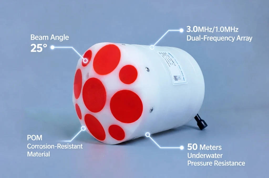
The PA5 uses a 5-beam phased-array transducer with a 30° beam angle and 3.5° beam width. Four beams are electronically steered in a Janus pattern; the fifth is a vertical center beam that directly measures vertical velocity. The phased-array design gives the PA5 a flat transducer face with no protruding ceramic elements, which reduces flow disturbance when profiling within meters of a structure. The wider 30° beams also provide broader horizontal coverage per ping — useful for spatial averaging in open harbor basins.
4.2 Velocity Accuracy
Both instruments achieve ±0.3% of measured velocity ± 3 mm/s — matching the Teledyne RDI Workhorse 600kHz, the industry benchmark. Flow direction accuracy is ±2° across 0–360°. Velocity resolution is 1 mm/s, with a default range of ±5.0 m/s and a maximum of ±20.0 m/s — more than sufficient for tidal ports where peak spring-tide currents rarely exceed 3 m/s.
4.3 Profiling Range and Cell Size
| Parameter | FA4 & PA5 Shared Spec | Port Relevance |
|---|---|---|
| Cell Size | 0.5 m – 4 m (user-selectable) | 0.5–1 m for berth approach studies; 2 m for general harbor circulation |
| Number of Cells | 1 – 255 | 0.5 m × 255 cells = 127.5 m theoretical max profile |
| Profiling Range (Broadband) | 55 m | Covers full water column for 95%+ of port environments |
| Profiling Range (Narrowband) | 70 m | Extended range for deeper approach channels |
| Data Output Rate | 2 Hz (no BT) / 1 Hz (with BT) | Fast enough for vessel surveys at 4–6 knots |
4.4 Bottom-Tracking Range
Bottom-tracking measures vessel speed-over-ground by locking onto the seabed echo — essential for mobile surveys. The FA4 bottom-tracks from 0.8 m to 120 m; the PA5 from 0.7 m to 110 m. Both ranges exceed the profiling range with comfortable margin for all standard port depths. Bottom-track accuracy is ±0.3% ± 3 mm/s — the same as the water-current measurement.
4.5 Physical Specifications
| Parameter | Ocean-ADCP-600-FA4 | Ocean-ADCP-600-PA5 |
|---|---|---|
| Housing | Titanium alloy | Titanium alloy |
| Depth Rating (Standard) | 1,000 m (optional 3,000 / 6,000 m) | 1,000 m (optional 3,000 / 6,000 m) |
| Weight in Air | 3.5 kg (1,000 m rating) | ≤ 1.8 kg |
| Dimensions (excl. connector) | Φ148 × 150 mm (1,000 m rating) | Φ92 × 112 mm |
| Average Power | ≤ 10 W | ≤ 5 W |
| Internal Storage | 64 GB Micro SD | 64 GB Micro SD |
| Communication | RS-232 or RS-422 | RS-232 or RS-422 |
| Operating Temp | −5°C to 45°C | −5°C to 45°C |
The physical differences are substantial. The PA5 weighs less than half what the FA4 does (≤1.8 kg vs. 3.5 kg), consumes half the power (≤5 W vs. ≤10 W), and is dramatically smaller — roughly half the diameter and three-quarters the height. For a port operator deploying on a cramped survey vessel or a diver installing a bottom mount in low visibility, these differences matter. The PA5’s lower weight and power draw make it the better choice for power-constrained DR installations (AUV/ROV) and space-limited permanent mounts. For autonomous SC deployments, the FA4-SC is the correct choice — the PA5 is DR only.
5. Step 4 — Pick the Right Instrument: FA4 vs. PA5
You now know your frequency (600kHz), your deployment type (DR or SC), and the specifications. Here is the direct comparison:
| Specification | Ocean-ADCP-600-FA4 | Ocean-ADCP-600-PA5 |
|---|---|---|
| Frequency | 600 kHz | 600 kHz |
| Beam Configuration | 4-beam Janus, convex, 20° angle, 3.5° beam width | 5-beam phased array, flat face, 30° angle, 3.5° beam width |
| Profiling Range | 55 m (broadband) / 70 m (narrowband) | 55 m (broadband) / 70 m (narrowband) |
| Bottom-Track Range | 0.8 – 120 m | 0.7 – 110 m |
| Velocity Accuracy | ±0.3% ± 3 mm/s | ±0.3% ± 3 mm/s |
| Flow Direction Accuracy | ±2° | ±2° |
| Vertical Velocity | Trigonometric derivation (4 beams) | Direct measurement (5th center beam) |
| Available Variants | DR + SC (separate instruments) | DR only |
| Housing | Titanium alloy | Titanium alloy |
| Depth Rating | 1,000 m (opt. 3,000 / 6,000 m) | 1,000 m (opt. 3,000 / 6,000 m) |
| Weight (Air) | 3.5 kg | ≤ 1.8 kg |
| Dimensions | Φ148 × 150 mm | Φ92 × 112 mm |
| Power Consumption | ≤ 10 W | ≤ 5 W |
| Storage | 64 GB Micro SD | 64 GB Micro SD |
| Data Rate | 2 Hz (no BT) / 1 Hz (with BT) | 2 Hz (no BT) / 1 Hz (with BT) |
When to Choose the FA4
The Ocean-ADCP-600-FA4 is the workhorse for general port monitoring. Its 4-beam, 20° Janus configuration is the global standard — the narrow beam angle produces a tighter seabed footprint, ideal for confined channels and near-structure deployments. The DR variant powers externally for cabled surveys and real-time stations; the SC variant runs on an internal battery delivering 100+ days of autonomous logging. For most port authorities, consulting firms, and survey contractors, the FA4 — in the variant that matches your deployment type — is the pragmatic choice.
When to Choose the PA5
The Ocean-ADCP-600-PA5 is the higher-performance option where size, weight, power, and vertical velocity accuracy drive the decision. Its 5-beam phased-array transducer with flat face and 30° beams provides direct vertical velocity measurement — valuable in ports with significant vertical flows near structures. The wider 30° beam also gives broader horizontal coverage per ping for open-harbor spatial averaging. At ≤1.8 kg and ≤5 W, it is the clear choice for AUV/ROV integration, space-constrained permanent installations, or any cabled deployment where minimizing payload weight and power draw is critical. The PA5 is available in DR variant only — if your port requires autonomous long-term bottom-mounted monitoring, select the FA4-SC.
6. How Ocean-ADCP-600 Compares to Alternative Products
| Evaluation Criterion | Ocean-ADCP-600 Series | Teledyne RDI Workhorse 600 | Nortek Signature 500/1000 | SonTek ADP 500 |
|---|---|---|---|---|
| True 600kHz Option | ✅ Yes — FA4 + PA5 | ✅ Yes — industry benchmark | No 600kHz — 500 or 1000kHz only | No 600kHz — 500kHz closest |
| Velocity Accuracy | ✅ ±0.3% ± 3 mm/s — matches Workhorse | ✅ ±0.3% ± 3 mm/s | ✅ ±0.3% ± 2 mm/s (rated) | ⚠ ±0.5% ± 2 mm/s (rated) |
| 5-Beam (Direct Vertical Velocity) | ✅ PA5 — phased array, flat face, 30° beams | 4-beam only at 600kHz | ⚠ Sig1000 has 5th beam — but 1000kHz limits port depth | 3-beam only |
| Titanium Housing | ✅ Standard on FA4 + PA5 | ⚠ Premium upgrade | ⚠ Premium upgrade | Plastic only |
| Standard Depth Rating | ✅ 1,000 m (opt. 6,000 m) | ⚠ 200 m standard | ⚠ 300 m standard | ⚠ 200 m standard |
| Onboard Storage | ✅ 64 GB | ⚠ 4 GB standard | ✅ 64 GB | ⚠ 16 GB |
| Price Positioning | ~2/3 of Workhorse equivalent | Premium benchmark | Premium tier | Mid-to-premium tier |
Two structural observations:
- Several major brands don’t make a 600kHz instrument. Nortek’s Signature series skips 600kHz entirely — the 500kHz has range overkill and resolution undershoot for ports; the 1000kHz has great resolution but range too short for turbid port water beyond ~25 m. SonTek’s ADP tops out at 500kHz. If 600kHz is your correct frequency, your options narrow before you compare prices.
- The Ocean-ADCP-600 matches the Workhorse on velocity accuracy (±0.3% ± 3 mm/s) and flow direction accuracy (±2°) at roughly two-thirds the cost. It ships with 64 GB of storage (vs. 4 GB), titanium as standard (vs. plastic with titanium as a paid upgrade), and a 1,000 m standard depth rating (vs. 200 m). The Workhorse has decades of field validation — but for a port authority choosing between one Workhorse or two Ocean-ADCP-600 units (one DR, one SC) at a comparable budget, the operational flexibility of dedicated instruments for each deployment type is a genuine advantage.
For ports operating AUVs or ROVs for underwater infrastructure inspection, the Oceantek DVL series provides 600kHz and 300kHz Doppler velocity logs sharing the same software ecosystem.
7. Data Quality in Port Environments: Sediment, Salinity & Tides
Regardless of which ADCP you select, port environments are acoustically challenging. Three factors dominate data quality:
7.1 Suspended Sediment and Acoustic Attenuation
High SSC from dredging, river inflow, and propeller wash attenuates the acoustic signal, reducing effective profiling range. A 600kHz ADCP rated for 55 m broadband / 70 m narrowband may see effective range drop by 20–30% during active dredging. Mitigation: the FA4 and PA5 both allow switching between broadband (higher temporal resolution) and narrowband (extended depth penetration). If your deployment coincides with dredging, run a range-validation test on day one — deploy, record actual range under real conditions, and adjust mode, cell size, and ping parameters before committing to a multi-week plan.
7.2 Salinity Gradients and Sound Speed Correction
Estuarine ports have spatially and temporally variable salinity. Freshwater overlying saltwater changes sound speed by up to 30 m/s through the water column. An uncorrected sound speed error introduces systematic bias — a single surface value applied to the entire profile can produce velocity errors of 1–2 cm/s, enough to corrupt a tidal harmonic analysis. Best practice: input a measured sound speed profile from a CTD or SVP cast at the deployment site. Both instruments include temperature sensors accurate to ±0.1°C. For multi-month deployments in strongly seasonal estuaries, schedule periodic CTD casts to update the sound speed model.
7.3 Tidal Sampling Strategy
In tidal ports, currents reverse every ~6 hours, with peak velocities often exceeding 2 m/s in constricted channels. Ensemble interval: minimum 4 per hour (15 min); recommended 12+ per hour (5 min) to capture slack water timing accurately. Near slack water, when current speed drops toward the instrument’s noise floor, velocity errors become proportionally larger — the ADCP’s low-noise characteristics at low flow speeds directly determine harmonic analysis quality.
8. Port Monitoring Deployment Checklist
Phase 1: Pre-Deployment Planning
- Define monitoring objectives. Tidal characterization? Dredge plume tracking? Model validation? Siltation baseline? The objective determines strategy.
- Survey the deployment site. Water depth, bottom type, vessel traffic patterns, seabed hazards (cables, pipelines, wrecks).
- Select instrument and variant. 600kHz for 5–50 m depths. DR variant for vessel surveys or cabled stations; SC variant for autonomous bottom-mounted deployments. FA4 (4-beam, 20°) for general use; PA5 (5-beam, 30°, ≤1.8 kg, ≤5 W) if size/weight/power or direct vertical velocity are priorities.
- Design the mooring (SC deployments). Frame or TRBM, ballast weight (2–3× instrument buoyancy), acoustic release if recovery is uncertain.
- Plan the sampling strategy. Ensemble interval (5–15 min), number of cells (1–255), cell size (0.5–4 m), coordinate system. Choose broadband (55 m) or narrowband (70 m) based on port depth.
Phase 2: Deployment
- Pre-deployment bench test. Verify all beams fire, clock synced to UTC, 64 GB storage formatted, batteries fresh (SC variant), compass calibrated. Use the Oceantek ADCP Utility to confirm configuration.
- Measure the sound speed profile. CTD or SVP cast at the deployment location. Input profile via RS-232/422. Do not skip this in an estuarine port.
- Record deployment metadata. GPS position, water depth, UTC time, frame orientation. Photograph everything.
- Run a validation transect. If deploying SC bottom-mount, run a DR vessel transect across the mooring for cross-validation.
Phase 3: Data Quality Control
- First-recovery QC. Check file integrity, attitude sensor drift (> 0.2° roll/pitch or > 0.8° heading drift warrants investigation), battery voltage log, beam correlation, echo intensity.
- Flag bad data. Beam correlation < 70%, side-lobe interference, pitch/roll > 15°, fish aggregation in beams.
- Apply time-varying sound speed correction if salinity/temperature changed significantly during deployment.
- Tidal harmonic analysis for deployments > 29 days — separate tidal from residual currents.
| Deployment Duration | Sampling Interval | SC Endurance (FA4) | Data Volume |
|---|---|---|---|
| 1 week (dredge monitoring) | 5 min | 100+ days (ample margin) | ~200 MB |
| 1 month (tidal cycle) | 15 min | 100+ days (ample margin) | ~400 MB |
| 3 months (seasonal baseline) | 30 min | 100+ days (approaching limit; external battery recommended) | ~600 MB |
| 6+ months (observatory) | 30–60 min | External battery required | ~1.2 GB+ |
9. Frequently Asked Questions
Q: Why is 600kHz the best frequency for port monitoring ADCP?
600kHz ADCPs offer the optimal balance between profiling range (55 m broadband / 70 m narrowband) and vertical resolution (0.5–4 m cells) for depths of 5–50 m. 300kHz sacrifices resolution for depth you don’t need; 1200kHz loses range in turbid port water.
Q: What is the difference between the DR and SC variants?
The DR (Direct-Reading) variant is cable-powered via RS-232/422 (20–50 V DC), streams real-time data at up to 2 Hz, and has a compact housing for vessel mounting or cabled installation. The SC (Self-Contained) variant has an extended housing with an internal battery pack, logging autonomously to 64 GB onboard storage for 100+ days (extendable to 6+ months with an external battery). DR and SC are separate physical instruments — you cannot convert one into the other. The FA4 is available in both DR and SC variants. The PA5 is available in DR only.
Q: Can I use the same ADCP for vessel surveys and long-term bottom monitoring?
Not with a single physical unit — DR is built for cabled operation, SC for autonomous battery-powered logging. However, because both variants share the same acoustic platform and software (Oceantek ADCP Utility), your team benefits from one processing workflow, one spares inventory, and one training investment across both deployment types.
Q: How does high suspended sediment affect data quality?
High SSC reduces profiling range. 600kHz penetrates turbid water better than 1200kHz. If your deployment coincides with dredging, run a range-validation test on day one and consider switching from broadband (55 m) to narrowband (70 m) mode if range falls short.
Q: What is the difference between the FA4 and PA5?
The FA4 uses a 4-beam Janus configuration with 20° beams and a convex transducer — tighter seabed footprint, ideal for confined channels. The PA5 uses a 5-beam phased-array with 30° beams and a flat face — adds direct vertical velocity measurement via the center beam, plus dramatically smaller (Φ92×112 mm vs. Φ148×150 mm), lighter (≤1.8 kg vs. 3.5 kg), and lower power (≤5 W vs. ≤10 W). Both use titanium alloy housings. Both achieve ±0.3% ± 3 mm/s velocity accuracy. Choose the FA4 for general port monitoring (including all autonomous SC deployments); choose the PA5 (DR only) when you need the smallest footprint, lightest weight, lowest power draw, or direct vertical velocity data in cabled/vehicle-mounted applications.
Q: How much does a port monitoring ADCP system cost?
Ocean-ADCP-600 pricing is positioned at roughly two-thirds the cost of an equivalent Teledyne RDI Workhorse 600kHz. A complete budget should include the instrument, mounting hardware or mooring frame ($2,000–$8,000), vessel time, and data processing software. The Oceantek ADCP Utility is included free for Windows. The PA5 carries a price premium over the FA4 reflecting the phased-array transducer; both are substantially below legacy-manufacturer pricing for 600kHz instruments with equivalent accuracy.
Disclosure:The Ocean-ADCP-600 series is manufactured by Oceantek. Readers are encouraged to compare specifications across manufacturers and request demonstration units before procurement. Prices cited are indicative 2026 list prices and may vary by region, configuration, and distributor.
Further Reading: Ocean-ADCP-600-FA4 Product Page · Ocean-ADCP-600-PA5 Product Page · Ocean ADCP Full Series · Contact Our Technical Team