Quick Reference: Parameters at a Glance
| Parameter | ADCP-600-DR-FA4 | What It Affects |
|---|---|---|
| Acoustic Frequency | 600 kHz | Shorter range, higher resolution — optimized for shallow water |
| Number of Beams | 4, Janus Configuration | 3D velocity measurement with error-velocity diagnostics |
| Beam Angle | 20° | Horizontal coverage; side-lobe performance near boundaries |
| Beam Width | 3.5° | Spatial footprint at profiling depth |
| Profiling Range (Broadband) | 55 m | Standard-mode water column coverage |
| Profiling Range (Narrowband) | 70 m | Extended range for deeper shallow-water applications |
| Bottom Tracking Range | 0.8 m – 120 m | Depth range for vessel-referenced velocity measurement |
| Blanking Zone | 0.5 m – 4 m (adjustable) | Near-transducer blind region |
| Velocity Accuracy | ±0.3% ±3 mm/s | Measurement uncertainty; superior to 300 kHz-class instruments |
| Velocity Resolution | 1 mm/s | Smallest detectable velocity change |
| Cell Size | 1 – 255 (1 mm resolution) | Vertical resolution of depth cells |
| Sampling Rate | 2 Hz (no BT); 1 Hz (with BT) | Temporal resolution; motion tolerance |
| Heading Range | 0° – 360° | Direction measurement coverage |
| Temperature Sensor | -5°C to 45°C; ±0.1°C | Sound-speed correction accuracy |
| Pressure Sensor | Per depth rating; ±0.25% | Depth telemetry accuracy |
| Communication | RS-232 / RS-422 | Cable length; data throughput |
| Storage | 64 GB Micro SD | Onboard logging duration |
| Power Consumption | ≤ 10 W (average) | Battery runtime; thermal management |
| Power Input | 20V – 50V DC, 5A | Vessel/field power compatibility |
| Continuous Operation | ≥ 100 days | Maximum autonomous deployment window |
| Depth Rating (Housing) | 1000 m / 3000 m / 6000 m | Maximum deployment depth (model-dependent) |
| Weight (Air/Water, 1000 m) | 3.5 kg / 2.8 kg | Single-person handling; small-vessel mounting |
| Transducer Material | Titanium Alloy (standard) | Seawater corrosion resistance; acoustic impedance matching |
If you are familiar with ADCP specifications, the table above is your reference. If you want to understand what each parameter means in the field — and why 600 kHz is the right choice for shallow-water work — read on.
1. Why 600 kHz: The Shallow-Water Specialist
Every ADCP frequency sits on a trade-off. Lower frequencies travel farther but deliver coarser resolution. Higher frequencies resolve finer detail but attenuate faster. 600 kHz occupies the upper-middle register of the ADCP spectrum:
| Frequency Band | Typical Profiling Range | Best Application | Oceantek Model |
|---|---|---|---|
| 75 kHz | 400–800 m | Deep ocean, full water-column profiling | ADCP-75-DR-PA4 |
| 300 kHz | 100–160 m | Continental shelf, coastal engineering | ADCP-300-DR-FA4 |
| 600 kHz | 40–70 m | Rivers, estuaries, nearshore, harbors | ADCP-600-DR-FA4 |
At 600 kHz, the ADCP-600-DR-FA4 delivers a profiling range of 55 m in broadband mode and 70 m in narrowband mode. The shorter acoustic wavelength means the returned Doppler signal has higher frequency resolution per unit velocity — which is why the velocity accuracy improves to ±0.3% ±3 mm/s, noticeably tighter than the ±0.5% achievable at 300 kHz.
Why This Matters for You: If your surveys are consistently in water depths under 60 m — river gauging stations, estuary monitoring, harbor engineering, nearshore coastal profiling — a 600 kHz ADCP is the correct instrument. You are trading deep-water range (which you never use) for better velocity precision and smaller physical size (which you benefit from on every deployment).
2. Profiling Range: What 55 m / 70 m Covers (and What It Does Not)
The ADCP-600-DR-FA4 operates in two acoustic modes:
- 55 m (Broadband Mode) — Shorter transmit pulses with coded phase modulation, producing lower single-ping velocity noise. This is the daily-use mode for most surveys.
- 70 m (Narrowband Mode) — Longer coded pulses that sacrifice some velocity precision for additional range. Switch to this when water depth exceeds ~45 m and you need full water-column coverage.
In practical terms, 55 m covers almost all river discharge measurement scenarios. The world’s major rivers are deep — but their gauging sections rarely exceed 30–40 m. The Amazon at Óbidos, one of the widest and deepest gauging stations on Earth, is approximately 55–60 m deep at the thalweg. A 600 kHz instrument with 55 m broadband range can profile that entire water column in standard mode.
Why This Matters for You: Do not think of 55 m as a hard wall. It is the range at which the returned signal-to-noise ratio drops below a usable threshold in typical water conditions. In turbid, sediment-rich water (common in rivers and estuaries), you may get more range because suspended particles are stronger acoustic scatterers. In exceptionally clear, particle-poor water, you may get less. The narrowband fallback at 70 m gives you headroom for the clear-water case.
3. Blanking Zone: Starting at 0.8 m — Why the Lower Bound Matters
The ADCP-600-DR-FA4 has an adjustable blanking zone of 0.8 m. The minimum of 0.8 m is a meaningful number for shallow-water work. Compare this with the 2 m minimum blanking of the 300 kHz model — the 600 kHz instrument gets you 0.8 m closer to the transducer face.
The 600 kHz blanking performance sits between the 300 kHz mid-range instrument and a dedicated ultra-high-frequency river ADCP — which is precisely the trade-off you want: river-capable blanking without sacrificing the range needed for coastal transitions.
Why This Matters for You: If your work includes shallow rivers (<10 m), the 0.8 m blanking zone preserves usable data near the surface, where flow velocities are highest and most important for discharge calculation. In contrast, deploying a 300 kHz ADCP in 5 m of water wastes 40% of the water column to blanking.
4. Velocity Accuracy: Why ±0.3% at 600 kHz Beats ±0.5% at 300 kHz
This is the specification that separates the 600 kHz class from lower-frequency instruments. The ADCP-600-DR-FA4 achieves ±0.3% ±3 mm/s velocity accuracy — a meaningful step up from the ±0.5% ±5 mm/s of the 300 kHz model.
Why does higher frequency improve accuracy? The Doppler frequency shift for a given water velocity is directly proportional to the transmitted frequency. At 600 kHz, a 1 m/s water current produces twice the frequency shift that it does at 300 kHz — meaning the receiver is working with a larger, easier-to-measure signal for the same physical flow speed.
Here is how the accuracy difference translates in real measurements:
| Measured Velocity | ADCP-600 | ADCP-300 |
|---|---|---|
| 20 cm/s | ±0.6 mm + 3 mm = ±3.6 mm/s | ±1.0 mm + 5 mm = ±6.0 mm/s |
| 50 cm/s | ±1.5 mm + 3 mm = ±4.5 mm/s | ±2.5 mm + 5 mm = ±7.5 mm/s |
| 100 cm/s | ±3.0 mm + 3 mm = ±6.0 mm/s | ±5.0 mm + 5 mm = ±10.0 mm/s |
| 200 cm/s | ±6.0 mm + 3 mm = ±9.0 mm/s | ±10.0 mm + 5 mm = ±15.0 mm/s |
Why This Matters for You: In river discharge measurement, a 1 cm/s systematic velocity error integrated across a 200 m wide, 10 m deep cross-section can bias discharge by 20 m³/s or more. Over repeated measurements, that bias compounds into water resource management decisions. The improved proportional accuracy of the 600 kHz instrument reduces this systematic error for the moderate-to-high velocity environments where it is designed to operate.
5. Bottom Tracking from 0.8 m: Getting a Lock in Very Shallow Water
The ADCP-600-DR-FA4 tracks bottom from 0.8 m to 120 m. The 0.8 m shallow limit is notably tight — many 600 kHz-class instruments bottom out (pun intended) at 1.0–1.5 m before losing bottom lock.
Why this matters: in river transect surveys, the vessel typically approaches the bank in water shallower than 2 m before turning around. If the ADCP loses bottom track at 1.5 m, the last several meters of each transect rely on GPS referencing or extrapolation — both less accurate than a solid bottom track. Maintaining lock down to 0.8 m means fewer gaps at the transect edges.
The 120 m upper bound on bottom tracking far exceeds the 55–70 m water-profiling range. This means that in moderate depths (50–80 m), bottom tracking continues to provide reliable vessel velocity reference even when the water-column echo has attenuated beyond its usable range.
Why This Matters for You: Bottom tracking is your primary velocity reference. GPS-based alternatives introduce additional latency, heading-misalignment errors, and multi-path issues in confined waterways. An instrument that keeps bottom lock from 0.8 m to 120 m reduces the number of deployments where you must fall back to GPS.
6. Power: ≤ 10 W Means Practical Field Autonomy
The ADCP-600-DR-FA4 draws ≤ 10 W average power during continuous operation. This is lower than the typical 300 kHz instrument (which runs 15–25 W depending on configuration), because transmitting at higher frequency requires less acoustic power to achieve the same signal-to-noise ratio over a shorter path.
What 10 W means in concrete terms:
- Vessel-powered deployment: Negligible draw on a standard 100 Ah 24V battery bank — the ADCP could run continuously for over 200 hours without recharging (though other electronics on the survey vessel will dominate).
- Autonomous moored deployment: Combined with the ≥ 100-day continuous operation rating, a modest external battery pack can sustain the instrument for a full field season.
- USV/AUV integration: At 10 W, the ADCP is a minor consumer on a typical unmanned surface vehicle power budget, leaving more endurance for propulsion and telemetry.
Why This Matters for You: If you are deploying on a small survey vessel with limited power outlets, or on an autonomous platform where every watt-hour counts against mission duration, a 10 W ADCP is a practical choice. You do not need a dedicated generator or oversized battery bank just to power the current profiler.
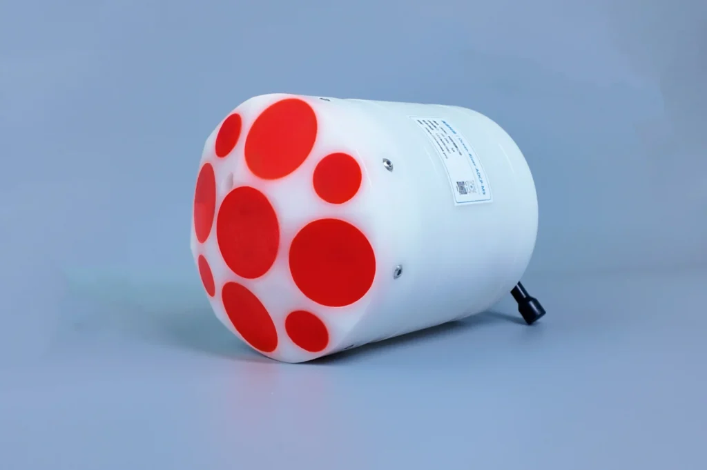
7. Physical Design: 3.5 kg in Air Changes How You Work
The ADCP-600-DR-FA4 weighs 3.5 kg in air / 2.8 kg in water (1000 m depth rating version) — roughly one-third lighter than its 300 kHz sibling and approximately half the weight of some competing 600 kHz instruments.
| Depth Rating | Weight (Air) | Weight (Water) | Typical Application |
|---|---|---|---|
| 1000 m | 3.5 kg | 2.8 kg | River survey, coastal monitoring, harbor engineering |
| 3000 m | 4.8 kg | 3.8 kg | Offshore energy, continental slope surveys |
| 6000 m | 5.7 kg | 4.6 kg | Deep-ocean ROV/AUV integration |
At 3.5 kg, the shallow-rated version is light enough for one person to mount on a pole or over-the-side bracket without assistance. This matters when you are working from a small boat with a two-person crew and every piece of equipment must be handled by one hand with the other hand holding onto the vessel.
The titanium alloy housing is standard across all depth ratings — the same material specified for deep-ocean instruments, applied to the entry-level model. Titanium provides galvanic compatibility with other underwater metals, corrosion resistance in warm saline water, and better acoustic impedance matching at the transducer-water interface compared to stainless steel or aluminum alternatives.
Why This Matters for You: Lighter weight = faster mobilization, fewer personnel, smaller mounting hardware, and reduced fatigue over a long survey day. The all-titanium construction also means you are not sacrificing material quality by choosing the shallow-rated version.
8. 600 kHz vs. 300 kHz: Choosing Between Oceantek’s Two Direct-Reading ADCPs
This is the most common question from buyers evaluating the Oceantek lineup. Both instruments share the same beam geometry (4-beam Janus, 20°), same data architecture (64 GB SD, RS-232/422), and same titanium construction. The difference is entirely in the acoustic frequency and what it enables:
| Decision Factor | ADCP-600-DR-FA4 | ADCP-300-DR-FA4 |
|---|---|---|
| Typical water depth | < 70 m | 70–150 m |
| Velocity precision | ±0.3% (better) | ±0.5% |
| Profiling range | 55 / 70 m | 120 / 160 m |
| Blanking zone (min) | 0.8 m (better for rivers) | 2.0 m |
| Weight (1000 m version) | 3.5 kg (lighter) | 5.3 kg |
| Power consumption | ≤ 10 W | ≤ 10 W |
| Best application | River discharge, estuary, harbor, aquaculture | Coastal engineering, shelf oceanography, offshore energy |
The short rule of thumb: If your surveys rarely exceed 70 m depth, pick the 600 kHz — you get better accuracy and a lighter instrument. If you regularly work between 70–150 m, the 300 kHz is the correct tool. If your work spans both ranges, the two instruments are complementary — the 600 kHz for the shallow/nearshore component and the 300 kHz for the deeper offshore component.
9. What These Numbers Do Not Tell You
Every datasheet has blank spots. Here is what the ADCP-600-DR-FA4 specifications page cannot communicate:
- How well the narrowband mode holds up in clear water. The 70 m specification assumes typical suspended sediment loads. In oligotrophic (nutrient-poor, low-particle) tropical waters, the real-world range will be shorter. In turbid river plumes, it may be longer. No manufacturer publishes a curve of range vs. turbidity — because it varies too much between sites.
- Velocity bias drift over time. The ±0.3% accuracy is a factory calibration figure. Long-term drift depends on transducer aging, electronics thermal cycling, and mechanical shock history. As a newer manufacturer, Oceantek is building the multi-year drift dataset that established brands already possess — and we encourage users to incorporate periodic reference checks into their deployment protocols.
- Software ecosystem compatibility. The ADCP-600-DR-FA4 outputs industry-standard binary and ASCII formats. But the quality of your data workflow — from acquisition software to post-processing to archival — is independent of the instrument hardware. Confirm that your preferred software stack (UHDAS, VmDas, WinRiver II, QRev, etc.) can ingest the data format before purchasing any ADCP, regardless of brand.
- What happens when you need help. A specification document does not tell you whether the manufacturer will answer your call from a survey vessel at 10 PM on a Saturday. We will — and we encourage you to test that before you commit.
Next Steps
If the ADCP-600-DR-FA4 looks suited to your survey program:
- Download the full datasheet — Contact sales@oceanadcp.com for the detailed product specification document with mechanical drawings and interface pinouts.
- Request a sample data file — Test a real-world dataset from a recent river or coastal deployment through your own processing chain.
- Ask about a loaner trial — In selected regions, we can arrange a short-term evaluation unit so you can run the instrument in your actual survey environment.
- Read our 600 kHz field report — See DVL-600K Qiandao Lake Test for a real deployment analysis of the 600 kHz acoustic platform.
- Compare the full product family — Visit our Direct-Reading ADCP product page to see the complete range (75 kHz, 300 kHz, 600 kHz).
Article last updated: June 2026. Specifications are subject to product improvement and may change. Contact Oceantek for the latest version.